Multiple Environmental Impacts of New
Infrastructure Investment Misallocation:
Evidence from China’s Industrial Structure

Kunjie Zhu; Simin Yang

doi:10.15244/pjoes/170800

About the Journal In Memory of Professor Jerzy Radecki Ownership and Management Statement Editorial Office Editorial Board Scope Impact Factor Indexed by Journal Impact Factor contributing items Publication Frequency Revenue Sources & Business Model Contact Subscription Journals Statistics Current issue Online first Instructions for Authors Copyright & Licensing Publication Fees Editorial policies Publication Policy Overview Peer Review Policy Research Ethics and Malpractice Policy Plagiarism Policy Conflict of Interest Policy Open Access Policy Instructions for Reviewers Generative AI and AI-Assisted Technologies Policy Advertising Policy Direct Marketing & Manuscript Solicitation Digital Archiving and Preservation Policy CrossMark, Correction, and Retraction Policy Complaints and Appeals Procedure Archive Publication Fees Copyright & Licensing

Current issue

Online first

Introduction, Research Background & Statistical Fact

Introduction

In the history of global economic development, the early extensive economic development model often brought considerable difficulties to the subsequent environmental governance. In the new economic era, the low-carbon and green economies have gradually become the recognized direction of future economic development [1, 2]. Since implementing the reform and opening-up policy, China has achieved remarkable economic achievements through traditional infrastructure construction. However, the environmental pollution caused by traditional infrastructure construction is also an unavoidable historical problem [3].

As China’s economy shifts from high-speed growth to high-quality development, the Chinese government has gradually increased its emphasis on green, low-carbon, and sustainable development. Unlike the U.S. government, which mainly uses the law as a means of environmental protection, the Chinese government has actively implemented a series of environmental protection policies and national green development plans [4]. Existing research proves that the Chinese-style environmental protection measures adopted by the Chinese government are highly effective. For example, measures such as new energy demonstration cities, civilized city construction, innovation-driven policies, and environmental protection tax laws have been proven to have made significant contributions to improving air pollution and industrial pollutant emissions [5-11]. However, China is not satisfied with the existing environmental protection achievements, and many environmental protection policies are still proposed and promoted yearly.

Compared with short-term environmental protection, the issue of economic recovery and industrial upgrading in the post-epidemic period is undoubtedly more critical. Therefore, in the special period when the government must maintain economic vitality, finding a more reasonable and efficient green governance measure has become a new problem.

At the same time, traditional infrastructure, which has made significant contributions in the stage of rapid economic growth, is also ushering in the historical process of iterative upgrading to new infrastructure in the stage of high-quality economic development. Traditional infrastructure is often considered to be an indisputable cause of today’s pollution problems. In contrast, new infrastructure with the characteristics of the digital economy and information economy is considered different from traditional infrastructure in this respect. As the hardware foundation of the digital economy, new infrastructure seems to be more environmentally friendly than traditional infrastructure. A report¹ jointly issued by international environmental protection organizations, the Renmin University of China, and other institutions pointed out that compared with traditional infrastructure, the carbon emissions of new infrastructure during the production process are also significantly lower than traditional infrastructure. In addition, from the perspective of data comparison, carbon dioxide emissions in the production process of the new infrastructure are reduced by 13.483 million tons compared with traditional infrastructure, and the emission reduction rate is about 7.24%. However, even though the research on the environmental impact of new infrastructure is still preliminary, society has already set high expectations for environmental protection.

In addition to environmental protection, the new infrastructure’s role in industry upgrading and transformation has also begun to attract attention from authoritative research institutions. While the development of the next generation of information technology and the digital economy promotes the upgrading of the industrial structure [12, 13], the new infrastructure which is the foundation of the former is naturally considered to have the same effect. On January 8, 2023, the “New Infrastructure Blue Book: China’s New Infrastructure Development Report (2022)” released by the Chinese Academy of Social Sciences, stated that new infrastructure had become a key highlight for major developed countries to stimulate economic growth. The report believes that the huge development potential and industry synergy contained in the new infrastructure provide unprecedented opportunities for future economic transformation. Society places high positive expectations on the role of the new infrastructure in industrial upgrading and the environmental impact.

Research Background

With the continuous increase in policy support for new infrastructure construction, new infrastructure investment is about to enter a stage of explosive growth. China’s Electronics Information Industry Development Research Institute (CCID) released the “White Paper on New Infrastructure Development” as early as March 2020. According to the report, it is estimated that by 2025, direct investment in new infrastructure in seven significant fields will reach 10 trillion yuan and drive over 17 trillion yuan in investment accumulation. Seven major fields include 5G infrastructure, UHV, high-speed intercity railway and urban rail transit, new energy vehicle charging piles, big data centers, artificial intelligence, and the industrial Internet. In the post-epidemic period, relevant new infrastructure investment support policies have been continuously promoted across the country.

As a solid foundation for the development of the digital economy, new infrastructure has been included in the 2022 work reports of several cities, becoming an important hand in building a new engine of economic growth.2023 On January 5, 2023, the State-owned Assets Supervision and Administration Commission (SASAC) emphasized the need to step up investment in new infrastructure in 2023 in a conference to deploy the work of state-owned central enterprises. By then, a large amount of official capital will be involved and private forces will be mobilized to build new infrastructure.

However, misallocating infrastructure investment could lead to potential environmental problems. The Environmental Kuznets Curve (EKC) suggests that environmental degradation initially increases with economic development, but beyond a certain level of economic development, environmental quality improves. By examining the potential nonlinear relationship between economic growth and environmental impacts, the framework also provides guidance in analyzing the relationship between new infrastructure, industrial structure, and environmental issues. As we all know, large-scale social infrastructure construction is a double-edged sword [14]. Although it can stimulate local economic development to a certain extent, it may also have a negative impact on environmental quality. Although new infrastructure has become an imperative project for future development in the eyes of scientific research institutions and government departments, there is still very limited research on the allocation of new infrastructure investment and the resulting environmental pollution. As an infrastructure project with digital characteristics, new infrastructure still has the possibility of environmental pollution similar to traditional infrastructure. Therefore, in the process of promoting new infrastructure construction, if the scale of new infrastructure investment is blindly determined without considering the characteristics of the local industrial structure, this may bring unexpected ecological disasters.

Considering the possible mismatch between new infrastructure investment and industrial structure, this paper innovatively studies the coupling coordination degree between new infrastructure investment and industrial structure upgrade level and its impact on environmental pollutants. This paper explores the environmental effects of the matching degree between new infrastructure investment and industrial structure, which is expected to fill the research gap in related fields. Although the interaction between new infrastructure investment and industrial institutions is predictable, this does not prevent us from studying the coupling between the two. In fact, studying the level of coupling between investment and industry and the corresponding environmental impacts enables us to take a more macro view of the level of matching between the two and the external impacts.

At the same time, the research conclusions can also provide some suggestions and empirical basis for the relevant government to formulate policies, so this paper has certain theoretical and practical significance. In the era of the booming digital economy, a large number of developing countries are eager to rely on new technologies and infrastructure for an industrial upgrade. The China case has undoubtedly given a large number of countries that are participating or preparing for participation a chance to learn and refer to. This is one of the reasons why the research in this paper is also applicable to international cases.

Statistical Fact

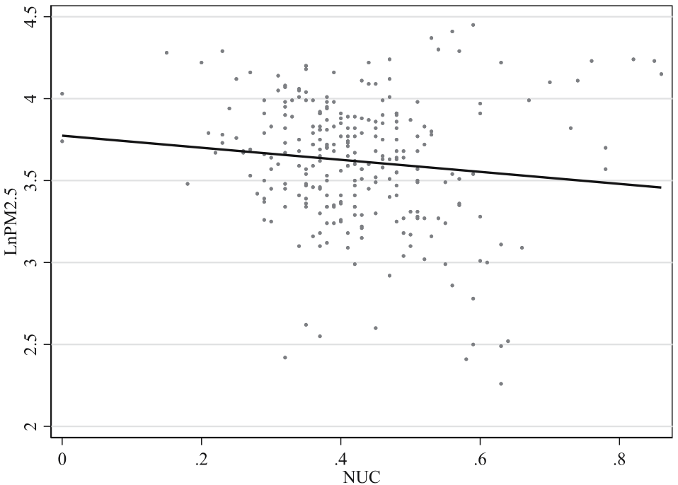
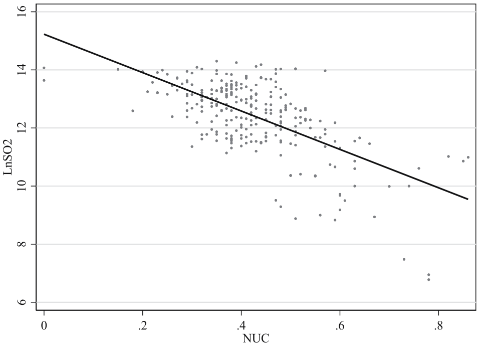
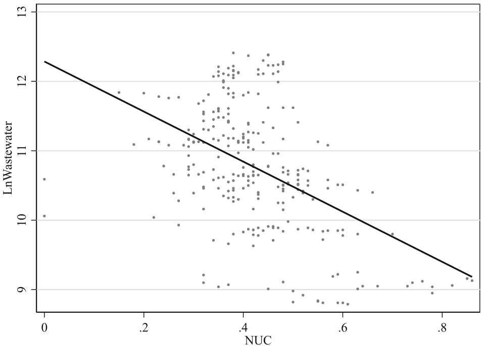
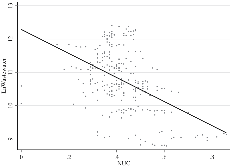
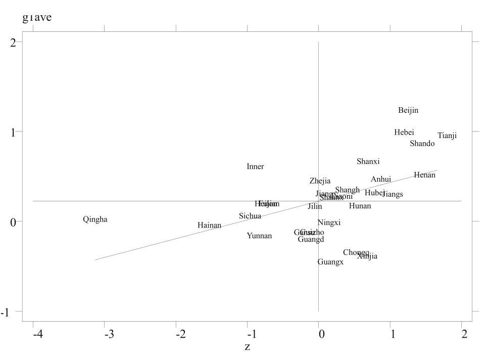
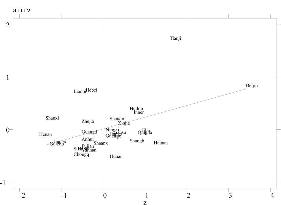
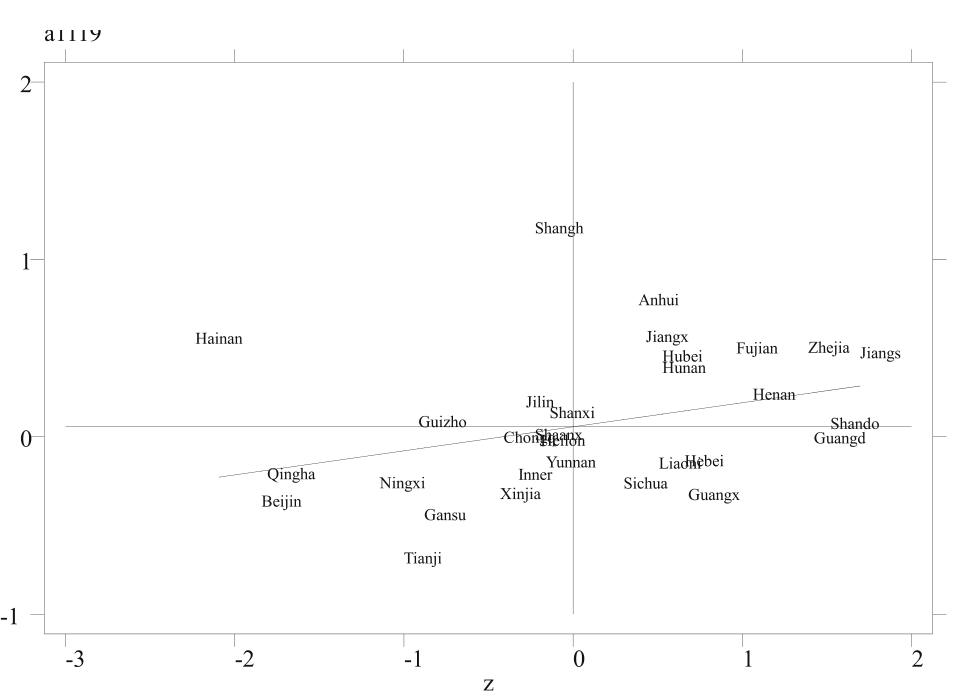
In addition to the evidence of previous literature, this study is also supported by strict statistical facts. As shown in the Figs 1-4², the matching degree of new infrastructure investment (NII) and industrial structure upgrading index (UIS) has a significant improvement effect on major environmental pollutants. The definition and quantification of NII and UIS will be given in the third part below. At the same time, this paper uses the coupling coordination degree to study the matching degree of NII and UIS, which is represented by NUC. In the selection of environmental pollutants, this paper mainly studies PM2.5, industrial wastewater discharge, industrial SO2 discharge and industrial dust discharge.

Literature Review, Hypothesis & Research Framework

Literature Review & Hypothesis

This paper mainly involves related literature on new infrastructure investment and industrial structure upgrading. For the part of new infrastructure investment, this section first introduces the definition and characteristics of new infrastructure and new infrastructure investment and sorts out the role of new infrastructure investment in industrial structure, environmental protection, energy structure, and green innovation. In the part of industrial structure upgrading, this paper introduces the primary quantitative standards of industrial structure upgrading and sorts out its environmental impact and energy effect. Based on the literature review results above, the article proposes a research hypothesis at the end of this section.

Fig. 1.

Relationship between NUC & PM2.5.

Fig. 3.

Relationship between NUC & SO₂

The New Infrastructure Investment (NII)

Since the concept of new infrastructure is still in the development stage, there are few relevant studies on the impact of existing new infrastructure. New infrastructure research has not yet been formed in T systematic and comprehensive system. In the limited literature, scholars’ existing research on new infrastructure and new infrastructure investment mainly focuses on its digital characteristics, multiple economic impacts, energy consumption, and environmental protection. In accordance with the main objective of the study, this paper emphasizes three aspects of literature: the concept of new infrastructure and new infrastructure investment, the impact of new infrastructure investment on industrial structure, and the impact of new infrastructure investment on the environment.

New infrastructure comes from traditional infrastructure, a concept that changes over time. As the name suggests, new infrastructure investment refers to investment funds for new infrastructure construction. The source of funds for new infrastructure investment mainly relies on fiscal funds and special bonds, and the investment scale of corporate and social funds is also increasing. With the continuous change of new technology, infrastructure content is constantly upgraded. Traditional infrastructure mainly includes elements that provide fundamental physical (public or private) services to industrial society: transportation, water, and wastewater treatment, electricity, and the military [14]. New infrastructure focuses more on infrastructure construction based on next-generation technologies.

Fig. 2.

Relationship between NUC & Wastewater.

Fig. 4.

Relationship between NUC & Smoke.

At present, new infrastructure research generally adopts the official answer of China’s National Development and Reform Commission as the definition of new infrastructure: new infrastructure is an infrastructure system guided by the new development concept, driven by scientific and technological innovation, based on the information network, and oriented by the demand for high-quality development, which provides digital transformation, intelligent upgrading, and convergence and innovation services. In addition, new infrastructure mainly includes three important aspects: information infrastructure, convergence infrastructure and innovation infrastructure. It should be noted that the so-called broadband infrastructure in the past was only part of the information infrastructure. The new infrastructure is a broader and more cutting-edge concept. Besides, China’s NDRC also emphasized that with technological revolution and industrial transformation, the connotation and extension of new infrastructure facilities will change. The official definition of new infrastructure reflects the development of new infrastructure construction itself, which also provides a more authoritative endorsement for the division benchmarks for quantifying new infrastructure investment in this paper.

Existing literature generally believes that new infrastructure can promote the upgrading of industrial structures. In fact, the new infrastructure investment can not only serve as an effective combination of stabilizing economic growth and optimizing economic structure [15], but also improve the quality of economic growth by stimulating technological innovation, optimizing industrial structure, and improving production efficiency [16]. In addition, the new infrastructure is the foundation of the digital economy, so it has a greater positive impact on the transformation and upgrading of industrial digitalization and informatization. The digital economy can promote the upgrading and transformation of the industrial structure [12, 17, 18], so the new infrastructure can also indirectly contribute to the transformation and upgrading of the industrial structure by supporting the growth of the digital economy.

Compared to traditional infrastructure, new types of infrastructure have been recognized as having environmental improvement effects due to their digital economy attributes. Existing literature on the environmental effects of new infrastructure investment generally focuses on green innovation and energy consumption. From the perspective of direct effects, the environmental effects of new infrastructure investment are mainly reflected in green innovation, green energy consumption and clean energy production. As part of the new infrastructure, the new digital infrastructure is considered to have a positive impact on the efficiency of green technology innovation in strategic emerging industries [19]. While promoting green energy consumption [20], the new infrastructure also opens up new development space and economic growth points for the clean energy industry. For example, intelligent energy construction related to new infrastructure is developing rapidly [21]. From the perspective of indirect effects, the close relationship between new infrastructure, the digital economy, and information technology will also drive corresponding environmental impacts. For example, the digital economy can accelerate the reduction of energy consumption intensity through economic growth, R&D investment, human capital, financial development, and industrial structure upgrading [22], so new infrastructure investment may also have a similar environmental protection effect. It is believed that information technology reduces energy demand by maximizing energy efficiency and changing sectors [23], and that digitalization can improve energy consumption and energy intensity, and optimize the energy structure [24]. New infrastructure may also contribute to environmental protection in similar ways.

The Upgrading of Industrial Structure (UIS)

Different from new infrastructure investment, the environmental protection effect, and energy impact of industrial structure upgrading have been confirmed by a large number of sources. Due to the focus of this paper, this part won’t repeat them. Overall, the upgrading of industrial structure helps to improve the efficiency of green development [25] and ecological efficiency [26] and can reduce environmental pollution [26-31]. In addition, UIS can also improve energy efficiency or energy intensity [2, 26, 31, 32].

For indicators of industrial structure upgrading, the literature often uses indicators such as the proportion of non-agricultural industries, the level coefficient of industrial structure, the ratio of the output value of the tertiary industry to the secondary industry, the Moore structural change index, and the proportion of high-tech industries [33]. As the coupling object of UIS, NII has been proven to have the effect of industrial structure upgrading and transformation [15, 16, 34], and new infrastructure investment has an upgrading effect on traditional manufacturing and service industries [15, 35]. In addition, considering that the research direction of this paper is environmental issues, adding the endogenous impact of agriculture will interfere with the empirical results. Therefore, this study uses the ratio of the tertiary industry’s output value to the secondary industry’s output value to measure the industrial structure upgrading index (UIS).

Hypothesis

Based on the above statistical fact and literature review, this paper makes the following hypotheses:

Hypothesis (H1). The degree of coupling and coordination between new infrastructure investment and the upgrading of industrial structure will have an impact on the local quality of environment.

Hypothesis (H2). The degree of coupling and coordination between new infrastructure investment and the upgrading of industrial structure has an impact on the energy consumption structure and the level of green innovation.

Research Framework

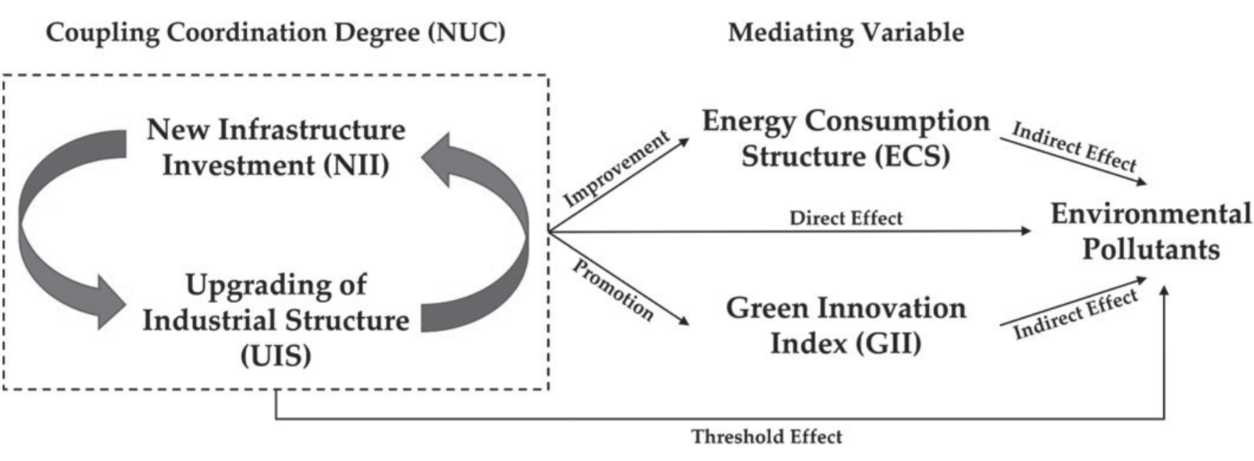
The research framework for this paper is divided into the following steps. Firstly, starting from the characteristics of new infrastructure investment (NII) and industrial structure upgrading (UIS), this paper studies the spatiotemporal dynamic distribution and spatial spillover effects of NII, UIS, and coupling coordination level (NUC). After that, the environmental effects of NUC are studied from both the perspective of direct impacts, as well as the perspective of indirect impacts, using the two mediator variables, energy consumption structure (ECS) and green innovation index (GII). Finally, based on the differences in the environmental impact results of direct and indirect effects, this paper explores the threshold effect of NUC on some environmental pollutants.

Fig. 5.

The Environmental Impact Mechanism Framework of NUC.

Methods of Research

Global Principal Component Analysis (GPCA)

In order to make the data comparable at the global sequence level, this paper adopts the global principal component analysis (GPCA) method to calculate the new infrastructure investment index (NII). In order to better reflect the information of multi-dimensional indicators, this paper chooses the time-series global principal component analysis (GPCA) method at the level of specific index construction, which can better reflect the overall characteristics of indicators. Specific practices refer to previous literature [36-38]. Through the global processing and calculation of ten third-level indicators, the new infrastructure investment index of the corresponding province in a certain year is obtained. Firstly, the three-level original indicators are standardized and the time-series global principal component analysis is used to reduce the dimension. Firstly, the three-level original index is standardized and the dimension is reduced by time-series global principal component analysis. Then, according to the principle that the cumulative variance contribution rate is not less than 85%, the number of principal components is determined and the score of each component is calculated. Finally, the final regional new infrastructure investment index is obtained by weighted summation of the principal component scores.

The Coupling Coordination Degree Model (CCDM)

In this paper, the degree of coupling coordination is used to represent the degree of matching between NII and UIS. The calculation of coupling degree refers to the concept of capacity coupling in physics and the capacity coupling coefficient model. The specific formula of coupling coordination degree is shown below:

(1)

Cn=2×[UNII·UUIS(UNII+UUIS)2]1/2

(2)

T=αUNII+βUUIS (α+β=1)

(3)

D=C·T

C_n represents the degree of coupling, U_NII and U_UIS represents the new infrastructure investment index (NII) and the index of upgrading of industry structure (UIS), respectively. The coordination degree is expressed by the coordination index T, which reflects the process of continuous harmony between the whole system or subsystems. D reflects the degree of coupling coordination between NII and UIS.

Global Spatial Autocorrelation Analysis (SAR)

Spatial statistics generally use the spatial autocorrelation index to reflect spatial dependence, and the research on the spatial dimension of coupling is gradually being valued by more and more environment-related research [39, 40]. By studying the spatial relationship of coupling coordination degree between new infrastructure investment and the upgrading of industry structure, this paper will help to observe the overall trend and dynamic distribution of coupling data across time and space. The specific operation mainly reflects the degree of aggregation through Moran index calculation, and its calculation formula is shown below.

(4)

Moran′s I=∑i−1n∑j≠inWij(xi−x¯)(xj−x¯)S2∑i=1n∑j=1nWij

(5)

S2=1n∑i=1n(xi−x¯)2x¯=1n∑i−1nxi

MI represents Moran index, and the value range of MI is [−1,1]. MI>0 indicates that the attribute values of spatial units are clustered and present as spatial positive autocorrelation; MI<0 indicates that the attribute values of spatial units are scattered and present as spatial negative autocorrelation; MI = 0 indicates that the attribute values of spatial units present as spatial random distribution. W_ij is a spatial weight matrix constructed based on spatial distance by using Stata software. N represents the total number of regional spatial units, x_i and x_j represent the attribute values of random variable x in geographic unit i and j, and is the average value of attribute values.

Threshold Regression Model (TR)

In order to test the nonlinear effect of NUC on pollutants under the condition of heterogeneity, the threshold model proposed by Hansen [41] is used for further analysis and research. The specific threshold regression model is set as follows:

(6)

yit=β0+β1xit×I(qit⩽γ)+β2xit×I(qit>γ)+εit

In the formula, I(·) is the indicative function, which takes the value of 1 when the conditions in the brackets hold, and 0 when the conditions in the brackets do not hold; qt is the threshold variable; y represents the unknown threshold value. In this paper, the expression can be rewritten as:

(7)

Lnwastewaterit=α0+α1×Mit×I(Lngdpi2it⩽q)+α2×Mit×I(Lngdpi2it>q)+α3Xit+εit

(8)

Lnsmokeit=β0+β1×Mit×I(Lneccit⩽q)+β2×Mit×I(Lneccit>q)+β3Xit+εit

M_it can be represented by NUC. As shown in the above model, here only assumes that there is a threshold q. In fact, most of them are double thresholds or triple thresholds, and the model setting method is similar to this. The specific model design should be based on the specific situation. This paper chose a more suitable single-threshold model after multiple threshold regression attempts.

Data Series, Distribution Analysis & Sources

Variable Distribution & Data Source

The core variable of this paper is the coupling coordination degree (NUC) between new infrastructure investment (NII) and industrial structure upgrading index (UIS). Based on the focus of relevant research, this paper selects smog concentration (LnPM2.5), industrial wastewater discharge (LnWastewater), industrial sulfur dioxide discharge (LnSO2) and industrial smoke discharge (LnSmoke) for environmental pollutants. In the data selection of mediators, this paper uses the proportion of coal consumption to represent the energy consumption structure (ECS), and uses the number of green invention patents obtained by 10,000 people to represent the green innovation index (GII).

Based on previous research experience and the variable characteristics of this study, the following control variables are selected in this paper: regional gross product per capita (Lnrgdp), regional population size (Lnpopu), regional coal consumption (Lnecc), regional population density (Lnpop), the proportion of regional fiscal expenditure on science and technology (Lntech) and the proportion of primary industry output value (Lnpt1).

In terms of data sources, the data on new infrastructure investment (NII) comes from the “China Fixed Assets Statistical Yearbook” and “China Fixed Assets Investment Statistical Bulletin”, and the energy-related data comes from the “China Energy Statistical Yearbook”. Green invention patent data comes from Chinese Research Data Services (CNRDS). The smog concentration data in the environmental pollution data comes from the Socioeconomic Data and Application Center of Columbia University, and the other pollutant data come from the “China Environmental Statistical Yearbook”. Other macroeconomic data come from “China Statistical Yearbook”. All the variables involved in the nominal value in this paper are deflated with 2010 as the base period, so as to reduce the influence of price factors.

Table 1.

Distribution of Main Variables.

Variable	Abbr.	Obs	Mean	Std. Dev.	Min	*Max*
Lnnii	NII	270	1.32	0.36	0.52	2.28
Lnuis	UIS	270	4.77	0.38	3.97	6.26
nuc	NUC	270	0.42	0.12	0.00	0.86
Lnecs	ECS	270	4.42	0.57	0.69	5.51
Lngii	GII	270	0.17	0.22	0.01	1.43
LnPM_2.5	G1	270	3.62	0.39	2.26	4.45
LnWastewater	G2	270	10.76	0.92	8.79	12.41
LnSO₂	G3	270	12.43	1.26	6.78	14.30
LnSmoke	G4	270	12.60	0.99	8.01	14.40

Table 2.

Composition of NII Index.

Level I indicators	Level II indicators.	Level III indicators
New infrastructure investment (NII)	Investment in information infrastructure	(A1) Per capita fixed asset investment in information technology services
	Integrated infrastructure investment	(A2) Per capita fixed asset investment in mining industry * PII
		(A3) Per capita investment in manufacturing fixed assets * PII
		(A4) Per capita investment in fixed assets in construction * PII
		(A5) Per capita investment in fixed assets of health and social work * PII
		(A6) Per capita fixed asset investment in transportation, storage, and postal services * PII
		(A7) Per capita fixed asset investment in water conservancy, environment, and public facilities management industry * PII
		(A8) Per capita investment in fixed assets in the production and supply of electricity, heat, gas, and water * PII
		(A9) Per capita investment in fixed assets of public administration, social security, and social organizations * PII
	Investment in innovative infrastructure	(A10) Per capita fixed asset investment in scientific research and technology services

Metrics & Distribution Analysis

The New Infrastructure Investment Index (NII)

Table 2 gives the specific multi-level index composition of new infrastructure investment. The National Development and Reform Commission of China divides the new infrastructure into three parts: information infrastructure, integrated infrastructure, and innovative infrastructure. In this paper, the new infrastructure investment index contains a total of three correspond secondary indicators. Investment in information infrastructure is measured by per capita fixed asset investment in information technology services. Proportionality coefficient PII (Proportion of information and innovation investment in new infrastructure investment) consists of proportion of investment in information infrastructure and innovative infrastructure of total new infrastructure investment. In the part of integrated infrastructure investment, it is calculated by multiplying the portion of traditional infrastructure related to new infrastructure by PII, which represents integrated infrastructure investment. Investment in innovative infrastructure is represented by per capita fixed asset investment in scientific research and technology services. This paper innovatively uses PII to calculate the relevant fixed asset investment share in the aspect of integrated infrastructure investment. This calculation method can more intuitively reflect the investment proportion of the integration of traditional infrastructure and new infrastructure.

Based on the composition of the above indicators, this paper first standardized the three-level indicators, and then used the principal component analysis method (GPCA) to reduce the dimensionality of the above indicators to extract the main features. In the process of processing, a cumulative contribution rate of 85% is set for principal component screening and score calculation, and finally the new infrastructure investment index is calculated. The result is shown in Table 3.

Table 3 provides the new infrastructure investment index of 30 provinces and cities in China from 2011 to 2019, and Fig. 2 ³ reports the dynamic level distribution of the new infrastructure index of 30 provinces and cities in China from 2011 to 2019 by region. The following part will analyze and evaluate based on the perspective of the individual, overall and essential time points in turn.

(1) At the individual level, from the perspective of the average value of various provinces and cities from 2011 to 2019, the overall level of the new infrastructure investment index is at a relatively low stage, and the differences between regions are still very significant. The average new infrastructure investment index in Beijing, the first place, is as high as 3.08, while the new infrastructure index in Guizhou Province, the last place, is only 1.31. The highest rankings are Tianjin, Qinghai, Inner Mongolia, Beijing, and Heilongjiang, and the lowest rankings are Guizhou, Henan, Chongqing, Yunnan, and Sichuan.

Table 3.

Results of NII Measurements in China’s Provinces.

Region	2011	2012	2013	2014	2015	2016	2017	2018	2019	Mean	Rank
Tianjin	2.79	2.94	3.21	4.01	2.46	3.37	5.51	1.93	1.46	3.08	1
Qinghai	-1.20	-1.67	-1.49	-0.27	5.31	4.98	3.26	3.93	5.79	2.07	2
Inner Mongolia	2.87	2.30	3.06	5.37	0.78	0.97	1.67	0.62	0.55	2.02	3
Beijing	2.96	3.81	3.44	1.25	0.58	-0.53	0.14	0.90	0.75	1.48	4
Heilongjiang	0.25	1.59	2.02	0.94	0.40	1.12	1.18	2.49	3.25	1.47	5
Jilin	-0.70	0.75	0.60	1.09	1.72	1.95	2.69	2.97	0.33	1.27	6
Shaanxi	1.42	2.29	1.72	2.73	1.08	0.75	0.04	0.40	-0.30	1.13	7
Jiangsu	0.48	0.87	1.20	1.24	1.43	0.59	0.40	0.26	0.11	0.73	8
Shandong	-0.03	0.54	1.55	0.66	1.49	0.86	0.33	0.50	0.28	0.69	9
Xinjiang	1.08	0.18	-0.32	0.13	0.42	0.62	0.99	0.82	-0.18	0.42	10
Hunan	-0.28	-0.70	-0.58	-0.46	0.26	0.10	0.36	1.81	2.61	0.35	11
Ningxia	0.38	-1.11	-0.83	-0.02	0.69	1.01	2.13	0.65	-0.02	0.32	12
Gansu	1.39	0.67	1.17	1.01	0.13	0.54	-1.19	-0.98	-1.43	0.14	13
Fujian	0.23	0.02	-0.14	-0.57	0.12	0.13	0.07	1.05	0.12	0.11	14
Hainan	0.53	-0.17	-0.89	-0.95	-0.31	0.28	0.19	-0.66	-0.45	-0.27	15
Liaoning	1.11	1.58	0.85	0.85	0.33	-2.00	-1.93	-2.27	-1.98	-0.38	16
Guangxi	-0.66	-0.85	-0.62	-0.77	-0.81	-0.51	-0.53	-0.19	0.05	-0.54	17
Hebei	-1.15	-1.06	-0.80	-0.90	-1.33	-0.67	-0.45	-0.05	0.87	-0.62	18
Anhui	-1.21	-0.57	-0.54	-0.43	-0.23	-0.13	-0.67	-0.71	-1.09	-0.62	19
Shanghai	0.90	0.40	-0.29	-0.91	-1.07	-1.30	-1.33	-1.28	-1.16	-0.67	20
Zhejiang	-0.48	-1.04	-0.87	-0.87	-0.95	-0.92	-1.11	-1.18	-0.60	-0.89	21
Hubei	-0.83	-0.70	-1.01	-1.37	-1.39	-1.36	-1.01	-0.63	-0.32	-0.96	22
Guangdong	-0.34	-0.43	-0.78	-0.90	-1.19	-1.44	-1.34	-1.60	-1.41	-1.05	23
Jiangxi	-1.57	-1.45	-1.58	-1.44	-1.20	-0.86	-0.78	-0.54	-0.19	-1.07	24
Shanxi	-0.97	-0.72	-0.59	-1.15	-0.54	-0.46	-1.83	-2.03	-1.77	-1.12	25
Sichuan	-1.33	-1.51	-1.61	-1.56	-0.93	-1.28	-1.38	-0.94	-0.21	-1.20	26
Yunnan	-0.74	-0.97	-1.01	-1.49	-2.00	-0.96	-1.30	-1.50	-1.80	-1.31	27
Chongqing	-0.75	-0.74	-0.88	-1.47	-1.55	-1.66	-1.51	-1.91	-1.40	-1.32	28
Henan	-2.15	-1.93	-1.83	-1.70	-1.66	-1.42	-1.28	-0.94	-1.02	-1.55	29
Guizhou	-2.01	-2.32	-2.18	-2.06	-2.03	-1.76	-1.31	-0.92	-0.84	-1.71	30

(2) At the overall level, the level of China’s new infrastructure investment is certainly on the rise from 2011 to 2019, with an increase of 223.87% during the period. In addition, from a regional perspective, there are significant differences in the distribution of new infrastructure investment. The level of new infrastructure investment in the eastern region was far ahead of the central and western regions at the beginning of the research period. However, as time passed, the level of new infrastructure investment in the eastern region continued to decline and has been lower than that of the central and western regions since 2018. The level of new infrastructure investment in the central region was the lowest in the early stage, but it continued to rise during 2011-2014. Then, after fluctuating from 2014 to 2016, it rose sharply again in 2017 and was in the middle of the country in 2019. The level of new infrastructure in the western region dropped sharply in the early days, bottomed out in 2013, and then began to bottom out. The new infrastructure investment in the western region ushered in a substantial increase in investment from 2013 to 2016 and began to fall slightly to the lowest position in 2016.

Fig. 6.

Changes in NII by Region in China, 2011-2019.

Fig. 7.

Kernel Density Map of NII by Region.

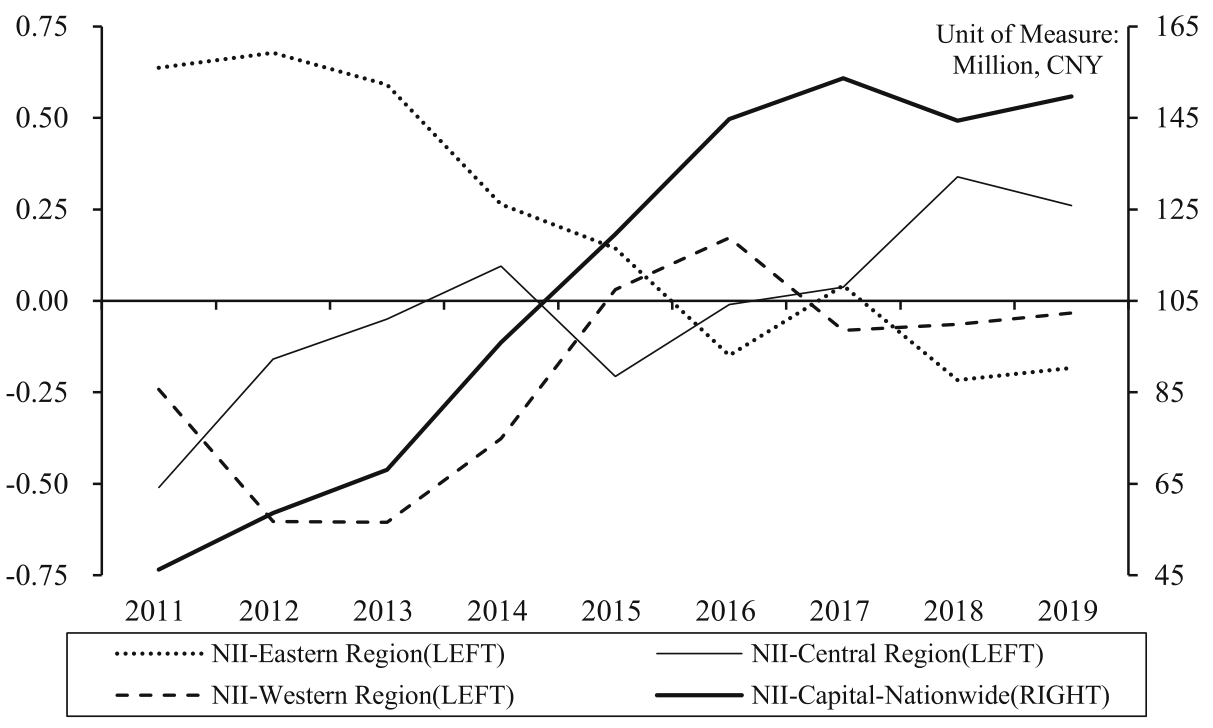
(3) At the primary time point level, the changes in the new infrastructure investment index of various provinces and cities are closely related to the macro policy and market environment. From 2008 to 2011, China launched a total of 4 trillion economic stimulus packages, which are considered to have significantly promoted the development of China’s infrastructure. After 2011, the impact of the four-trillion economic stimulus plan gradually weakened, which can be reflected in the new infrastructure investment capital in Fig. 6. In February 2013, the State Council of China issued the “National Major Science and Technology Infrastructure Construction Medium and Long-term Plan (2012-2030)”. The plan pointed out that by 2030, China will basically build a significant science and technology infrastructure with a complete layout, advanced technology, efficient operation, and strong support system. In November 2014, China’s National Development and Reform Commission and other units issued the “National Major Science and Technology Infrastructure Management Measures” to provide detailed regulations on the construction and operation management of major science and technology infrastructure. The above-mentioned policy emphasis on new infrastructure construction in China can be reflected in the substantial growth of new infrastructure investment capital from 2013 to 2017 in the Fig. above. For the central region, the State Council of China issued the “Several Opinions of the State Council on Vigorously Implementing the Strategy for Promoting the Rise of the Central Region” in August 2012, which mentioned that the future development of the central region needs to comprehensively strengthen the construction of public infrastructure and support private capital to enter the infrastructure field. This policy corresponds to the growth of the new infrastructure investment index in the central region from 2012 to 2014. In August 2013, the National Development and Reform Commission of China released the “Notice on the Progress of the Western Development in 2012 and the Work Arrangement in 2013”, emphasizing the acceleration of infrastructure construction in the western region, and proposed that the 2013 Western Development Develop new key projects, and do a good job in tracking and coordinating the progress of projects under construction. This policy provides a policy-side explanation for the substantial increase in new infrastructure investment in the western region from 2013 to 2016 in Fig. 6.

Table 4.

Results of UIS Measurements in China’s Provinces.

Region	2011	2012	2013	2014	2015	2016	2017	2018	2019	Mean	Rank
Beijing	3.79	3.90	4.03	4.14	4.57	4.77	4.89	5.02	5.23	4.48	1
Hainan	1.72	1.82	2.19	2.21	2.28	2.50	2.55	2.73	2.92	2.32	2
Shanghai	1.43	1.59	1.78	1.91	2.18	2.47	2.44	2.47	2.72	2.11	3
Tianjin	1.12	1.15	1.22	1.27	1.39	1.59	1.69	1.73	1.80	1.44	4
Jilin	1.26	1.26	1.29	1.29	1.28	1.38	1.46	1.49	1.52	1.36	5
Yunnan	1.13	1.12	1.19	1.24	1.35	1.46	1.56	1.53	1.50	1.34	6
Gansu	0.88	0.93	1.00	1.06	1.32	1.46	1.57	1.60	1.68	1.28	7
Qinghai	1.20	1.18	1.22	1.28	1.37	1.35	1.28	1.27	1.29	1.27	8
Guangxi	0.96	1.04	1.16	1.17	1.27	1.37	1.43	1.48	1.53	1.27	9
Guizhou	1.18	1.16	1.20	1.20	1.21	1.22	1.33	1.40	1.43	1.26	10
Heilongjiang	0.68	0.74	0.79	0.95	1.29	1.48	1.66	1.78	1.85	1.25	11
Xinjiang	0.77	0.87	1.03	1.05	1.29	1.37	1.35	1.39	1.47	1.18	12
Guangdong	0.93	0.99	1.03	1.04	1.11	1.22	1.28	1.32	1.39	1.15	13
Chongqing	1.05	1.02	1.02	1.01	1.08	1.16	1.22	1.29	1.35	1.13	14
Inner Mongolia	1.01	0.98	1.01	1.06	1.15	1.18	1.26	1.27	1.27	1.13	15
Liaoning	0.73	0.80	0.87	0.99	1.18	1.36	1.38	1.37	1.39	1.12	16
Hunan	0.86	0.88	0.92	0.96	1.04	1.16	1.29	1.39	1.35	1.09	17
Sichuan	0.82	0.85	0.87	0.94	1.02	1.17	1.31	1.40	1.42	1.09	18
Ningxia	0.91	0.96	1.00	1.03	1.10	1.15	1.10	1.17	1.19	1.07	19
Zhejiang	0.86	0.92	0.96	0.96	1.03	1.10	1.17	1.21	1.30	1.06	20
Hebei	0.82	0.85	0.89	0.92	1.02	1.06	1.15	1.26	1.35	1.04	21
Shandong	0.77	0.83	0.90	0.95	1.03	1.11	1.16	1.24	1.32	1.04	22
Jiangsu	0.82	0.86	0.92	0.97	1.02	1.09	1.09	1.11	1.17	1.01	23
Hubei	0.79	0.79	0.90	0.94	1.01	1.06	1.14	1.19	1.22	1.00	24
Anhui	0.76	0.77	0.80	0.84	0.98	1.07	1.14	1.23	1.27	0.98	25
Shanxi	0.53	0.61	0.69	0.78	1.13	1.19	1.07	1.15	1.16	0.92	26
Henan	0.64	0.69	0.74	0.78	0.84	0.91	0.94	1.07	1.13	0.86	27
Shaanxi	0.69	0.69	0.72	0.75	0.88	0.95	0.95	0.97	1.02	0.85	28
Fujian	0.76	0.76	0.76	0.75	0.81	0.87	0.94	0.93	0.98	0.84	29
Jiangxi	0.62	0.65	0.67	0.70	0.80	0.90	0.95	1.07	1.09	0.83	30

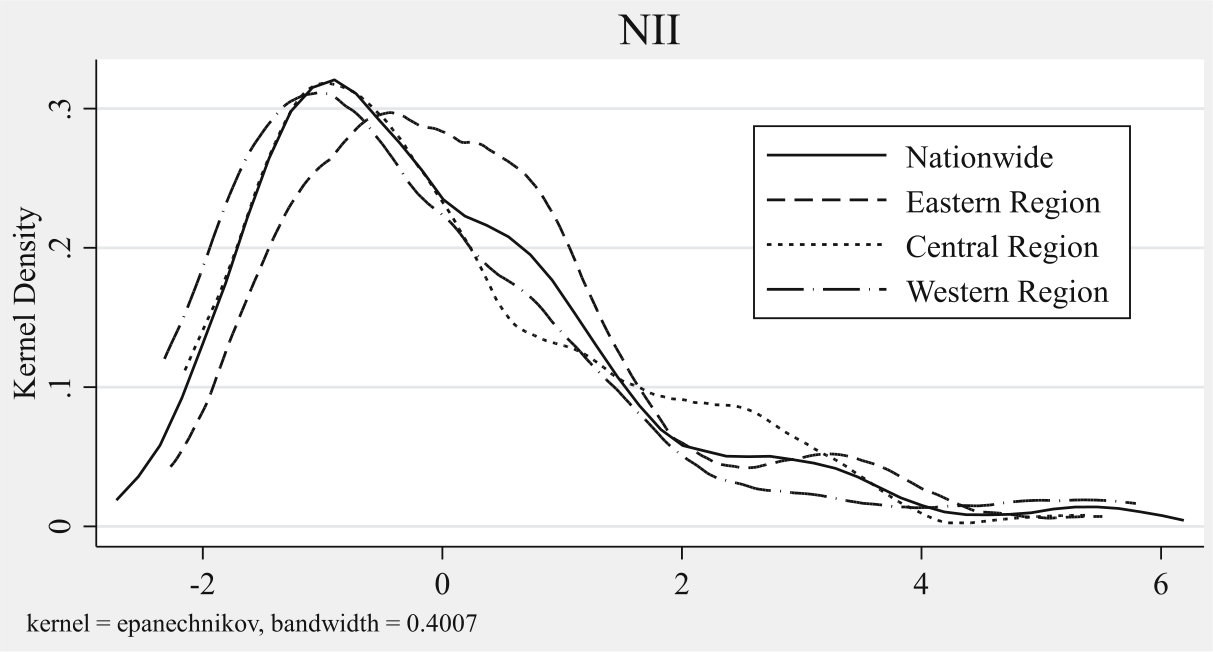
Fig. 7 shows the kernel density distribution map of the new infrastructure investment index as a whole and by region. First, from the perspective of the peak, the peak of the central and western regions is higher than that of the eastern region, which shows that the level of new infrastructure investment in the central and western regions is more concentrated. Secondly, from the perspective of curve distribution, the curve distribution in the eastern region is more to the right than in the central and western regions. Therefore, the level of new infrastructure investment in the eastern region is higher than that in the central and western regions. Finally, from the perspective of curve shape, the curve in the eastern region is relatively wider than that in the central and western regions. This shows that the regional differences in the new infrastructure investment level in the eastern region are relatively significant. In contrast, the regional gap in the new infrastructure investment index in the central and western regions is relatively small.

Fig. 8.

Changes in UIS by Region in China, 2011-2019.

Fig. 9.

Kernel Density Map of UIS by Region.

The Index of Upgrading of Industry Structure (UIS)

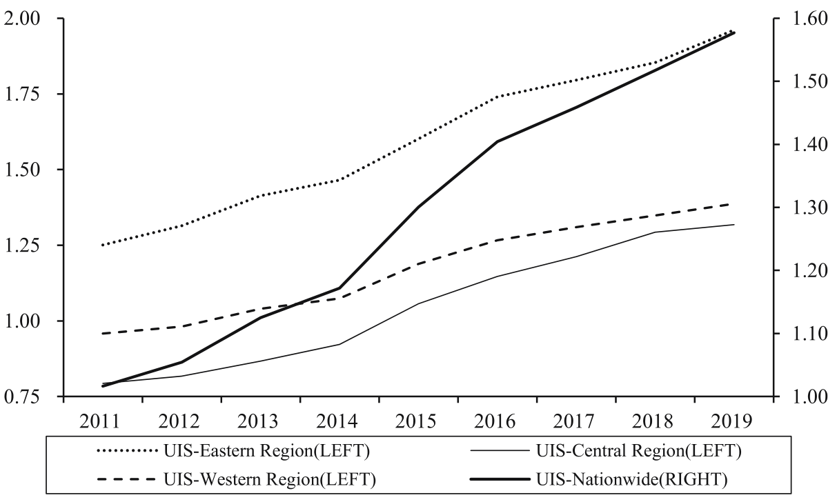
Table 4 specifically reports the industrial structure advanced index of China’s 30 provinces and cities during 2011-2019. Fig. 8 shows the dynamic distribution of the industrial structure advanced index of China’s 30 provinces and cities from 2011 to 2019 by region. In the following, the analysis and evaluation of the data based on the mean value and time-point changes are also carried out.

(1) From the average point of view, the overall level of the industrial structure upgrading index of China’s provinces and cities from 2011 to 2019 is at a relatively high stage. However, the differences between regions are significant. The average industrial structure upgrading index of Beijing, which ranks first, is as high as 4.48, while the industrial structure upgrading index of Jiangxi Province, which ranks last, is only 0.83. The top rankings are Beijing, Hainan, Shanghai, Tianjin, and Jilin, and the lowest are Jiangxi, Fujian, Shaanxi, Henan, and Shanxi.

(2) From the perspective of overall changes, it is evident that China’s industrial structure was in an upgrading trend from 2011 to 2019, during which the industrial structure upgrading index rose as high as 55.17%. However, from a regional perspective, there is no significant difference in the distribution of the industrial structure upgrading index. In the initial period, the level of new infrastructure investment in the eastern region was far ahead of the central and western regions during the study period. However, as time passed by, the three regions basically showed a similar upward trend, and after 2014, they all showed a similar acceleration trend.

(3) Judging from the primary time points, there is still a relatively large relationship between the changes in the industrial structure upgrading index of various provinces and cities in China and the policy environment. In 2014, the Chinese government emphasized the importance of the development of the service industry, accelerated the advancement of the industrial structure, and introduced related policies for this purpose. In 2014, China’s National Development and Reform Commission (NDRC) issued the newly revised “Industrial Structure Adjustment Guidance Catalog (2014 Version)”, which came into effect on June 1 of that year. Since 2014, the eastern, central, and western regions have all started an accelerated period of industrial structure upgrading, consistent with the trend of China’s industrial structure upgrading index after 2014 in Fig. 8.

Table 5.

Results of NUC Measurements in China’s Provinces.

Region	2011	2012	2013	2014	2015	2016	2017	2018	2019	Mean	Rank
Beijing	0.82	0.86	0.85	0.76	0.74	0.67	0.73	0.78	0.78	0.78	1
Tianjin	0.53	0.54	0.56	0.59	0.57	0.63	0.70	0.60	0.60	0.59	2
Hainan	0.55	0.52	0.50	0.50	0.55	0.61	0.60	0.56	0.59	0.55	3
Jilin	0.42	0.49	0.49	0.51	0.53	0.56	0.59	0.60	0.51	0.52	4
Qinghai	0.37	0.32	0.35	0.45	0.64	0.63	0.58	0.59	0.63	0.51	5
Inner Mongolia	0.51	0.48	0.51	0.57	0.47	0.49	0.53	0.49	0.49	0.50	6
Shanghai	0.53	0.52	0.51	0.48	0.48	0.48	0.47	0.48	0.51	0.49	7
Heilongjiang	0.32	0.39	0.42	0.43	0.48	0.54	0.57	0.63	0.66	0.49	8
Xinjiang	0.38	0.39	0.40	0.43	0.48	0.50	0.52	0.52	0.48	0.46	9
Gansu	0.43	0.42	0.46	0.46	0.48	0.51	0.42	0.44	0.40	0.45	10
Shandong	0.35	0.39	0.44	0.43	0.47	0.47	0.46	0.48	0.48	0.44	11
Jiangsu	0.38	0.41	0.44	0.45	0.47	0.46	0.45	0.45	0.45	0.44	12
Hunan	0.36	0.35	0.37	0.38	0.43	0.45	0.48	0.55	0.57	0.44	13
Ningxia	0.41	0.34	0.37	0.42	0.46	0.48	0.51	0.47	0.45	0.43	14
Guangxi	0.37	0.37	0.41	0.40	0.41	0.45	0.45	0.48	0.50	0.43	15
Shaanxi	0.36	0.37	0.38	0.41	0.42	0.43	0.40	0.42	0.40	0.40	16
Hebei	0.31	0.32	0.35	0.35	0.34	0.39	0.42	0.46	0.51	0.38	17
Yunnan	0.40	0.38	0.39	0.35	0.29	0.43	0.41	0.38	0.34	0.37	18
Fujian	0.35	0.35	0.34	0.32	0.37	0.39	0.40	0.43	0.41	0.37	19
Zhejiang	0.36	0.34	0.36	0.36	0.37	0.38	0.38	0.38	0.43	0.37	20
Guangdong	0.38	0.39	0.38	0.37	0.36	0.35	0.37	0.35	0.38	0.37	21
Anhui	0.29	0.32	0.34	0.35	0.40	0.42	0.40	0.41	0.39	0.37	22
Hubei	0.32	0.32	0.34	0.32	0.33	0.34	0.38	0.41	0.44	0.36	23
Liaoning	0.37	0.41	0.41	0.44	0.46	0.29	0.30	0.18	0.29	0.35	24
Sichuan	0.29	0.29	0.28	0.30	0.37	0.36	0.37	0.42	0.47	0.35	25
Chongqing	0.38	0.38	0.37	0.32	0.32	0.32	0.35	0.30	0.37	0.35	26
Jiangxi	0.21	0.23	0.23	0.25	0.30	0.35	0.36	0.40	0.42	0.30	27
Guizhou	0.27	0.00	0.22	0.26	0.27	0.32	0.38	0.42	0.43	0.29	28
Shanxi	0.00	0.24	0.29	0.30	0.41	0.42	0.29	0.26	0.31	0.28	29
Henan	0.15	0.20	0.23	0.25	0.27	0.31	0.33	0.37	0.38	0.28	30

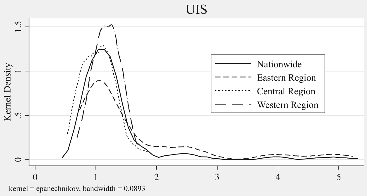
Fig. 9 shows the kernel density distribution map of the industrial structure upgrading index as a whole and by region. As for the peak angle, the peak in the western region is higher than that in the central region, and the peak in the eastern region is the lowest. This shows that the upgrading level of industrial structure in the western region is more concentrated, while the upgrading level in the eastern region is more scattered. From the perspective of curve distribution, the curve distribution of the western region is more to the right than that of the eastern and central regions, so the industrial structure upgrading level of the western region is higher than that of the eastern and central regions. Finally, comparing the shape of the curve, the curves in the eastern and central regions are broader than those in the western region, which shows that the regional differences in the upgrading level of industrial structure in the eastern and central regions are relatively significant. In contrast, the regional differences in the upgrading level of industrial structure in the western region are relatively small.

Fig. 10.

Changes in NUC by Region in China, 2011-2019.

The Coupled Coordination Index of NII & UIS (NUC)

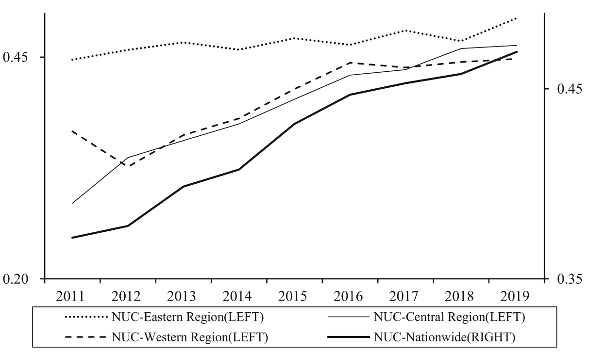
In this study, the coupling coordination degree represents the matching degree between NII and UIS. This part uses the coupling coordination degree formula to calculate the coupling coordination degree of NII and UIS. For the coupling coordination standard, this paper divides the whole into five standards: high incoordination (0-0.2), moderate incoordination (0.2-0.4), basic coordination (0.4-0.6), and moderate coordination (0.6-0.8) and high coordination (0.8-1). From the perspective of the overall coupling coordination level, the coupling coordination level of the 30 provinces and cities in China is generally at a relatively low level, and there are currently no provinces and cities in China that are in the stage of high NUC coordination. At the level of indicator differences, there are currently significant differences in NUC between provinces and cities in China. Beijing, which ranks first, is 0.78, while Henan, which ranks last, is 0.28. The top provinces and cities of NUC are Beijing, Tianjin, Hainan, Jilin, and Qinghai, and the bottom provinces and cities are Henan, Shaanxi, Guizhou, Jiangxi, and Chongqing.

Fig. 10 shows the NUC index’s global and regional division timing changes. Overall, China’s national NUC level has been rising since 2011 and is gradually approaching 0.5 in a basic coupling state. From the perspective of regional division, the NUC in the east is significantly higher than that in the west and central regions. Then the gap between the three is continuously narrowing, and they are already at the same level of coupling & coordination standards. The NUC in the central and western regions was still moderately uncoordinated in 2011 but entered a basic coordinated state in 2019.

The trend of NUC in Fig. 10 has a certain relationship with China’s local economic policies. From 2011 to 2019, the Chinese government vigorously promoted upgrading the industrial structure in the central and western regions. The main measures in the government policy include the increase of infrastructure construction and the construction of major scientific and technological infrastructure, which corresponds to the impact of the previous policy on new infrastructure investment and NUC. The Chinese government’s emphasis on investment in new infrastructure and technological infrastructure in the central and western regions has continuously promoted the rise of NUC levels in the central and western regions, consistent with the trend in Fig. 10.

Fig. 11.

Kernel Density Map of NUC by Region.

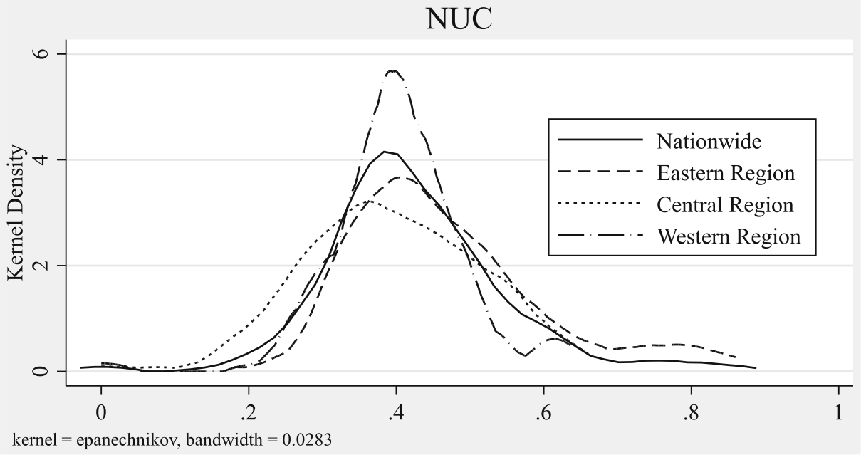
Table 6.

Spatial Moran Index of NII, UIS, NUC & Pollutants.

Variables	2011	2012	2013	2014	2015	2016	2017	2018	2019	Mean
nii	0.199*** (2.876)	0.281*** (3.895)	0.303*** (4.151)	0.185*** (2.835)	0.097** (1.718)	0.01 (0.57)	0.004 (0.501)	0.009 (0.535)	-0.024 (0.143)	0.228*** (3.22)
uis	-0.009 (0.498)	-0.008 (0.511)	-0.009 (0.461)	-0.007 (0.494)	-0.009 (0.466)	0.004 (0.67)	0.015 (0.866)	0.006 (0.721)	0.006 (0.686)	0.003 (0.689)
nuc	0.117** (2.002)	0.163*** (2.674)	0.232*** (3.659)	0.31*** (4.418)	0.233*** (3.358)	0.157*** (2.346)	0.199*** (2.886)	0.039 (0.926)	0.096* (1.639)	0.223*** (3.357)
g1	0.194*** (2.919)	0.147*** (2.33)	0.211*** (3.093)	0.252*** (3.644)	0.26*** (3.725)	0.237*** (3.425)	0.206*** (3.095)	0.186*** (2.756)	0.177*** (2.692)	0.208*** (3.092)
g2	0.138** (2.101)	0.143** (2.162)	0.148** (2.238)	0.152** (2.281)	0.166*** (2.455)	0.113** (1.804)	0.105** (1.704)	0.096* (1.597)	0.115** (1.83)	0.136** (2.081)
g3	0.011 (0.594)	0.01 (0.567)	0.01 (0.568)	0.007 (0.529)	0.013 (0.618)	0.102** (1.735)	0.063* (1.295)	0.074* (1.455)	0.065* (1.338)	0.041 (0.981)
g4	0.079* (1.47)	0.06 (1.212)	0.062 (1.238)	0.079* (1.455)	0.101** (1.745)	0.06 (1.189)	0.029 (0.806)	0.039 (0.929)	0.081* (1.604)	0.055 (1.139)

Fig. 11 presents the kernel density distribution plot of the NUC index overall and by region. At the peak level, the peak in the western region is higher than that in the eastern region, and the peak in the eastern region is higher than that in the central region. This shows that the NUC level in the western region is more concentrated, while the NUC level in the eastern region is more scattered. The most dispersed region in the NUC index is still the central region. In terms of curve distribution, the curve distribution in the eastern and western regions is more to the right than in the central region, so the NUC levels in the eastern and western regions are higher than those in the central region. Finally, from the perspective of curve shape, the curves in the eastern and central regions are wider than those in the western region, which indicates that the regional differences in NUC levels in the eastern and central regions are relatively large. In contrast, the regional differences in NUC levels in the western regions are relatively small.

Empirical Results and Discussion

Spatiotemporal Effect & Distribution Character

The literature has proved that environmental pollution has a particular spatial effect. Considering that the research object of this paper may also have spatial attributes, this paper chooses to study the spatial properties related to NUC and environmental pollutants. In order to better display the characteristics of NII, UIS, NUC, and pollutants, this paper conducts a spatial autocorrelation analysis based on the square term matrix of geographic distance for the above variables. Table 6 reports the spatial effects of the variables in each year and the mean from 2011 to 2019. The results show significant spatial spillover effects in NII, NUC, G1, and G2 but not in UIS, G3, and G4. From a time series perspective, the spatial spillover effect of NII has gradually decreased. It has not been significant since 2016, while the spatial spillover effects of NUC, G1, and G2 are significant, and the Moran index level is relatively stable.

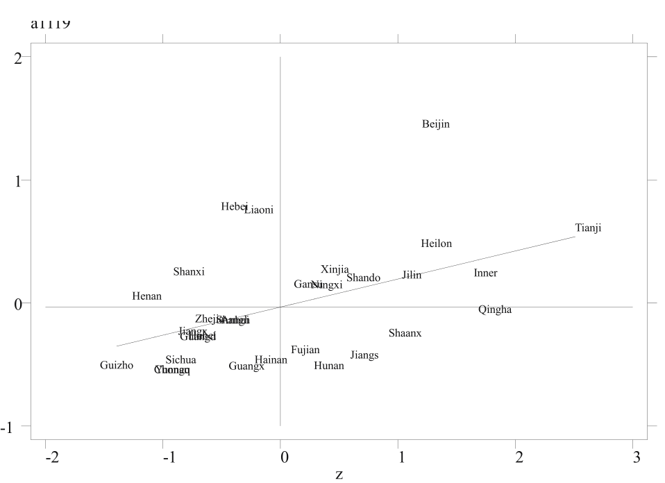
Figs 12-15 show Moran’s index plots for NII, NUC, G1 and G2. The distribution in the figure shows that there is a significant positive spatial autocorrelation in the spatial distribution of the above variables, and it mainly manifests as “high-high” and “low-low” clusters. This proves that there is a significant positive spatial correlation between investment in new infrastructure and the degree of coupling between investment in new infrastructure and the upgrading of industrial structure. At the same time, the concentration of PM2.5 in pollutants and the discharge of industrial wastewater also have spatial spillover properties.

Multiple Impact Effects of NUC on Environmental Pollution

The Direct Effect Analysis

Table 7 shows the current and lagged individual fixed effect regression⁴ results of NUC on the primary pollutants PM2.5, industrial wastewater discharge, industrial sulfur dioxide discharge and industrial dust discharge in the panel data of 30 provinces and cities in China from 2011 to 2019. Regression (1) showed that NUC significantly reduced the concentration of PM2.5, and the coefficient was significant at the 1% level. Specifically, when nuc increases by 0.1 units, the haze level decreases by 9.53%. Regression (2) shows that NUC significantly reduces the discharge of industrial wastewater, and the coefficient is significant at the 5% level. When nuc increased by 0.1 unit, sewage discharge decreased by 5.34%. Regression (3) shows that NUC significantly reduces industrial SO2 emissions, and the coefficient is significant at the 1% level. When NUC increased by 0.05 units, industrial sulfur dioxide emissions decreased by 23.5%. Regression (4) shows that NUC significantly reduces industrial dust emissions, and the coefficient is significant at the 5% level. When NUC increased by 0.1 unit, industrial sulfur dioxide emissions decreased by 8.07%. Considering that NUC and other control variables may have a hysteresis effect on the impact of environmental pollutants, the individual fixed effect analysis of the lagged one period in regression (5)-(8) in Table 7. The results show that NUC has a significantly lagged negative impact on PM2.5, industrial sulfur dioxide emissions and industrial dust emissions, and the conclusion is more significant than the same period regression, both at the 1% significance level. Moreover, the hysteresis influence coefficient of NUC on g1 and g4 is higher than the same period influence coefficient, which shows that the lag influence of NUC on the improvement of PM2.5 and industrial dust emissions is stronger than the current influence. At the same time, regression (6) shows that the lagged effect of NUC on industrial wastewater discharge is not significant in the fixed effect regression.

Fig. 12.

Moran index scatterplot for NII.

Fig. 14.

Moran index scatterplot for G1.

Fig. 13.

Moran index scatterplot for NUC.

Fig. 15.

Moran index scatterplot for G2.

Robustness Test of the Direct Effect

Table 8 shows the results of the 2SLS robustness test of the regression of NUC on individual fixed effects of pollutants. Regression (1)-(4) uses the 2SLS method to test the robustness of the environmental impact of NUC in the current period, and selects NUC with a lag of one period as the instrumental variable for regression. In the regression of environmental effects on NUC in the current period, the impact coefficients of NUC on g1~g4 are all negative, and they are all significant at the 1% confidence level. This shows that NUC does have an improving effect on the current impact of environmental pollutants, and the conclusion has certain reliability. Regression (5)-(8) used the 2SLS method to test the robustness of the NUC environmental effect with a lag of one period, and also selected NUC with a lag of two periods as an instrumental variable for regression. In the regression of the environmental effect of NUC with a lag of one period, the impact coefficients of NUC on g1, g3 and g4 were all negative and significant at the 1% confidence level. This shows that NUC does have a certain time-lag effect on the improvement of environmental pollutants g1, g3 and g4, and the conclusion has certain reliability. However, the regression results of NUC on Wastewater (g2) are similar to the results of the fixed effect with a one-period lag, and they are not significant. This shows that NUC cannot reduce industrial wastewater discharge.

Table 7.

The Fixed Effect Regression of NUC’s Impact on the Pollutants.

Variables	(1)	(2)	(3)	(4)	(5)	(6)	(7)	(8)
	FE	(2)	(3)	(4)	FE-LAG	(6)	(7)	(8)
	g1	g2	g3	g4	g1	g2	g3	g4
nuc	-.953***	-.534**	-4.715***	-.807**
	(.265)	(.25)	(1.293)	(.387)
Lnrgdp	-.927***	.685	-3.467*	.067
	(.268)	(.515)	(1.819)	(.704)
Lnpopu	-1.761***	.254	-11.658***	-.761
	(.565)	(.427)	(3.191)	(1.273)
Lnecc	.204***	.221**	1.474***	.757***
	(.04)	(.093)	(.273)	(.205)
Lnpop	-.166	-.028	-.832	-.029
	(.107)	(.087)	(.551)	(.214)
Lntech	-.08	.081	.41	.31
	(.092)	(.138)	(.5)	(.221)
L_nuc					-.961***	-.359	-4.585***	-1.154***
					(.247)	(.257)	(1.136)	(.362)
L_Lnrgdp					-.49	.654	.866	2.314***
					(.316)	(.576)	(1.753)	(.719)
L_Lnpopu					-2.222***	.831	-15.211***	-1.647*
					(.65)	(.555)	(3.04)	(.85)
L_Lnecc					.293***	.246***	1.965***	1.028***
					(.052)	(.086)	(.272)	(.217)
L_Lnpop					-.146	.084	-.647	.367
					(.108)	(.138)	(.572)	(.257)
L_Lntech					-.054	.031	.44	.539*
					(.11)	(.162)	(.589)	(.276)
Individual	Fixed	Fixed	Fixed	Fixed	Fixed	Fixed	Fixed	Fixed
_cons	27.526***	-.057	138.288***	11.405	25.769***	-5.616	116.573***	-10.185
	(5.915)	(7.307)	(36.22)	(11.452)	(7.82)	(9.289)	(39.231)	(11.681)
Observations	270	270	270	270	240	240	240	240
r2_w	.471	.086	.504	.174	.434	.071	.542	.283

[i] Note: Based on robust standard error. *** p<.01, ** p<.05, * p<.1

Table 9 shows the results of the IV-GMM robustness test for the regression of NUC on individual fixed effects of pollutants. Regression (1)-(4) uses the IV-GMM method to test the robustness of the environmental impact of NUC in the current period, and chooses NUC with a lag of one period as the instrumental variable for regression. In the regression of environmental effects on NUC in the current period, the impact coefficients of NUC on g1~g4 are still negative, and they are all significant at the 1% confidence level. This shows that the current impact of NUC on environmental pollutants does improve, and the conclusion is robust. Regression (5)-(8) uses the 2SLS method to test the robustness of the NUC environmental effect with a lag of one period, and selects NUC with a lag of two periods as an instrumental variable for regression. In the regression of the environmental effect of NUC with a lag of one period, the impact coefficients of NUC on g1, g3 and g4 are all negative, and the regression of NUC on g1 and g2 is significant at the 1% confidence level, and the regression on g4 is at 5 Significant at the % level. This shows that NUC does have a certain time-lag effect on the improvement of environmental pollutants g1, g3 and g4, and the conclusion has certain reliability. However, the regression results of NUC on g2 are similar to the results of fixed effects and 2SLS with a one-period lag, and they are not significant. This shows that NUC does not reduce industrial wastewater discharge.

Table 8.

2SLS Robustness Test of NUC’s Impact on the Pollutants.

Variables	(1)	(2)	(3)	(4)	(5)	(6)	(7)	(8)
	2SLS	(2)	(3)	(4)	2SLS-LAG	(6)	(7)	(8)
	g1	g2	g3	g4	g1	g2	g3	g4
nuc	-1.493***	-.741***	-7.858***	-2.218***
	(.234)	(.263)	(1.172)	(.662)
Lnrgdp	-1.139***	.777**	-4.583***	-.194
	(.249)	(.394)	(1.461)	(.769)
Lnpopu	-1.309***	.759**	-10.649***	-.541
	(.424)	(.355)	(1.752)	(.978)
Lnecc	.214***	.218***	1.557***	.817***
	(.031)	(.049)	(.186)	(.201)
Lnpop	-.193***	.002	-.922***	-.129
	(.07)	(.077)	(.329)	(.185)
Lntech	.018	.161	.925***	.573***
	(.073)	(.103)	(.349)	(.208)
L_nuc					-1.859***	-.33	-8.534***	-2.752***
					(.298)	(.428)	(1.319)	(.765)
L_Lnrgdp					-.633**	.636	.142	2.494***
					(.315)	(.455)	(1.592)	(.864)
L_Lnpopu					-2.307***	1.201***	-14.714***	-1.786*
					(.46)	(.418)	(1.759)	(1.018)
L_Lnecc					.352***	.233***	2.169***	1.171***
					(.053)	(.056)	(.303)	(.199)
L_Lnpop					-.233***	.113	-.928***	.209
					(.079)	(.125)	(.343)	(.17)
L_Lntech					.127	.099	1.087**	.775***
					(.09)	(.115)	(.432)	(.235)
Individual	Fixed	Fixed	Fixed	Fixed	Fixed	Fixed	Fixed	Fixed
_cons	27.971***	-6.754	143.214***	12.686	29.257***	-9.69	116.422***	-13.262
	(4.185)	(5.251)	(20.971)	(11.159)	(5.125)	(6.042)	(22.506)	(12.492)
Observations	240	240	240	240	210	210	210	210
R-squared	.906	.959	.785	.867	.903	.957	.799	.881

[i] Note: Based on robust standard error. *** p<.01, ** p<.05, * p<.1

The Mediating Effect Analysis – ECS & GII

This section presents evidence for the mediating effects of NUC on environmental pollutants. Table 10 shows the results of the mediating effect mechanism of NUC affecting major pollutants by improving the energy consumption structure and increasing the level of green innovation. Regression (1) shows that NUC can reduce the proportion of coal consumption in the energy consumption structure, and the result is significant at the 5% level. For every 0.1 unit of NUC, the proportion of coal consumption will decrease by 2.57%. Regression (2)-(5) results show that the proportion of coal consumption (Lnecs) does have a mediating effect on pollutants g1, g2, g3 and g4 in NUC. Among them, NUC can reduce the pollution levels of g1, g3 and g4 by improving the energy consumption structure, and the results are established within the 1% confidence interval. As for the industrial sewage discharge g2, NUC increased the industrial sewage discharge level by improving the energy consumption structure. Specifically, from a quantitative perspective, the indirect impact of NUC on g1 by improving energy consumption is -2.57*0.511 = -1.3133; the indirect impact on g2 is -2.57*-0.312 = 0.8018; the indirect impact on g3 is -2.57*2.678 = -6.8825; the indirect effect on g4 is -2.57*1.172 = -3.012. Regression (6) shows that NUC can improve the level of local green innovation, and the result is significant at the 5% level. For every 0.1 unit of NUC, the level of green innovation will increase by 2.00%. Regression (7)-(10) results show that the level of green innovation (Lngii) does have a mediating effect in the mechanism of NUC’s impact on pollutants g1, g2, g3 and g4. Among them, NUC can reduce the pollution level of g1, g2 and g3 by improving the level of green innovation. The results of g1 and g3 are established in the 1% confidence interval, and the results of g2 are established in the 5% confidence interval. As for industrial dust emission (g4), NUC cannot improve the dust emission problem by improving the quality of green innovation. Specifically, from a quantitative perspective, the indirect impact of NUC on g1 by improving the level of green innovation is 0.2*-.843 = -0.1686; the indirect impact on g2 is 0.2*-.407 = -0.0814; the indirect impact on g3 is 0.2* -5.974 = -1.1948.

Table 9.

The Fixed Effect Regression of NUC’s Impact on the Pollutants.

Variables	(1)	(2)	(3)	(4)	(5)	(6)	(7)	(8)
	IV-GMM	(2)	(3)	(4)	IV-GMM-LAG	(6)	(7)	(8)
	g1	g2	g3	g4	g1	g2	g3	g4
nuc	-1.493***	-.741***	-7.858***	-2.218***
	(.25)	(.281)	(1.253)	(.708)
Lnrgdp	-1.139***	.777*	-4.583***	-.194
	(.266)	(.422)	(1.562)	(.822)
Lnpopu	-1.309***	.759**	-10.649***	-.541
	(.453)	(.38)	(1.872)	(1.045)
Lnecc	.214***	.218***	1.557***	.817***
	(.033)	(.053)	(.199)	(.215)
Lnpop	-.193**	.002	-.922***	-.129
	(.075)	(.083)	(.352)	(.197)
Lntech	.018	.161	.925**	.573**
	(.078)	(.11)	(.373)	(.223)
L_nuc					-3.096***	-.362	-15.025***	-3.84**
					(.459)	(.949)	(2.065)	(1.609)
L_Lnnii					.679***	.13	3.579***	.874**
					(.109)	(.205)	(.508)	(.373)
L_Lngdp					-.946***	.572	-1.937	1.579
					(.274)	(.527)	(1.425)	(1.087)
L_Lnpopu					-.86	.637	-10.565***	-3.296**
					(.579)	(.787)	(2.595)	(1.523)
L_Lnfdi					.013	.009	.018	-.013
					(.01)	(.012)	(.052)	(.031)
L_Lntech					-.007	.04	.529	.653**
					(.074)	(.134)	(.365)	(.255)
Individual	Fixed	Fixed	Fixed	Fixed	Fixed	Fixed	Fixed	Fixed
Observations	240	240	240	240	210	210	210	210
R-squared	.392	.092	.409	.117	.552	.046	.565	.135

[i] Note: Based on robust standard error. *** p<.01, ** p<.05, * p<.1

Table 10.

The Fixed Effect Regression of NUC’s Impact on the Pollutants.

Variables	(1)	(2)	(3)	(4)	(5)	(6)	(7)	(8)	(9)	(10)
	Lnecs-FE	(2)	(3)	(4)	(5)	Lngii-FE	(7)	(8)	(9)	(10)
	Lnecs	g1	g2	g3	g4	Lngii	g1	g2	g3	g4
nuc	-.257**	-.822***	-.614**	-4.028***	-.506	.2**	-.963***	-.364	-3.855***	-.31
	(.124)	(.252)	(.257)	(1.206)	(.362)	(.09)	(.221)	(.273)	(.88)	(.396)
Lnecc	.895***	-.254	.5***	-.924	-.292	-.108***	.078	.146	.246	.313
	(.09)	(.157)	(.163)	(.881)	(.339)	(.029)	(.074)	(.104)	(.405)	(.244)
Lnpop	-.051	-.14	-.044	-.696	.031	.058	-.16	.007	-.702	.021
	(.062)	(.098)	(.085)	(.461)	(.174)	(.035)	(.102)	(.093)	(.416)	(.172)
Lnrgdp	-.342	-.752***	.578	-2.551	.468	-.049	-1.052***	.813	-3.014**	.591
	(.203)	(.225)	(.522)	(1.674)	(.672)	(.125)	(.222)	(.502)	(1.248)	(.6)
Lnpopu	-2.045***	-.714	-.384	-6.18*	1.636
	(.345)	(.707)	(.566)	(3.63)	(1.293)
Lntech	.013	-.087	.085	.376	.295
	(.071)	(.087)	(.134)	(.477)	(.189)
Lnecs		.511***	-.312*	2.678***	1.172***
		(.164)	(.173)	(.915)	(.399)
Lnpt1						-.011***	-.003	.003	.067*	.061***
						(.003)	(.007)	(.014)	(.037)	(.009)
Lngii							-.843***	-.407*	-5.974***	-1.213
							(.262)	(.22)	(1.42)	(.796)
Individual	Fixed	Fixed	Fixed	Fixed	Fixed	Fixed	Fixed	Fixed	Fixed	Fixed
_cons	16.943***	18.861***	5.23	92.917**	-8.45	1.144	15.514***	1.219	49.157***	3.69
	(3.253)	(6.433)	(7.99)	(38.823)	(12.742)	(1.404)	(2.5)	(5.462)	(13.714)	(6.831)
Observations	270	270	270	270	270	266	266	266	266	266
r2_w	.913	.509	.095	.545	.208	.258	.479	.099	.627	.248

[i] Note: Based on robust standard error. *** p<.01, ** p<.05, * p<.1

Table 11.

Robustness Test of the Mediating Effect.

Variables	(1)	(2)	(3)	(4)	(5)	(6)	(7)	(8)	(9)	(10)
	Lnecs+2SLS	(2)	(3)	(4)	(5)	Lngii+2SLS	(7)	(8)	(9)	(10)
	Lnecs	g1	g2	g3	g4	Lngii	g1	g2	g3	g4
nuc	-.347***	-1.31***	-.898***	-7.063***	-1.845***	.317***	-1.358***	-.438*	-6.214***	-1.427**
	(.087)	(.223)	(.284)	(1.182)	(.679)	(.064)	(.197)	(.24)	(.811)	(.628)
Lnecc	.935***	-.278*	.64***	-.583	-.188	-.047	.116*	.134*	.389	.333
	(.056)	(.145)	(.171)	(.699)	(.361)	(.058)	(.067)	(.07)	(.327)	(.3)
Lnpop	-.077*	-.152**	-.032	-.747**	-.047	.052**	-.183**	.05	-.823***	-.064
	(.042)	(.061)	(.076)	(.29)	(.175)	(.022)	(.071)	(.081)	(.268)	(.157)
Lnrgdp	-.417***	-.919***	.589	-3.628***	.254	-.013	-1.153***	1.107***	-3.338***	.771
	(.125)	(.216)	(.388)	(1.38)	(.777)	(.075)	(.207)	(.391)	(1.106)	(.651)
Lnpopu	-1.925***	-.294	-.111	-6.241***	1.528
	(.199)	(.555)	(.483)	(2.361)	(1.263)
Lntech	.041	-.004	.18*	.832**	.529***
	(.038)	(.069)	(.101)	(.338)	(.205)
Lnecs		.527***	-.452***	2.29***	1.075**
		(.152)	(.161)	(.797)	(.438)
Lnpt1						-.013**	-.004	.01	.077**	.068***
						(.006)	(.01)	(.009)	(.031)	(.026)
Lngii							-.775***	-.409**	-5.919***	-1.3*
							(.163)	(.169)	(.742)	(.695)
Individual	Fixed	Fixed	Fixed	Fixed	Fixed	Fixed	Fixed	Fixed	Fixed	Fixed
_cons	16.407***	19.322***	.664	105.641***	-4.948	.967	19.462***	-3.789	62.184***	2.701
	(1.867)	(4.664)	(5.5)	(24.234)	(13.741)	(.873)	(2.375)	(4.427)	(12.358)	(7.669)
Observations	240	240	240	240	240	236	236	236	236	236
R-squared	.992	.914	.96	.804	.873	.941	.915	.959	.852	.881

[i] Note: Based on robust standard error. *** p<.01, ** p<.05, * p<.1

Table 12.

Heterogeneity Test Based on Threshold Effect.

Threshold	Lngdpi2	Lnecc
Variables	(1)	(2)
Variables	g2	g4
0bn._cat#c.nuc	-.516**	-.228
	(.244)	(.302)
1._cat#c.nuc	.334	-2.103***
	(.312)	(.376)
Control	Yes	Yes
Individual	Fixed	Fixed
_cons	1.812	4.459
	(7.269)	(10.331)
Observations	270	270
R-squared	.138	.25

[i] Note: Based on robust standard error. *** p<.01, ** p<.05,

[ii] * p<.1

Robustness Test of the Indirect Effect

From the perspective of robustness, the regressions (1) and (6) in Table 11 are the results of the 2SLS robustness test of NUC on the regression of Lnecs and Lngii fixed effects, respectively. Regression (2)-(5), (7)- (10) in Table 11 correspond to the 2SLS robustness test results of the mediating effects of Lnecs and Lngii in the NUC environmental pollution impact mechanism, respectively. The results passed the insufficient identification of instrumental variables and weak instrumental variable tests, indicating that the use of instrumental variables is reasonable and the use of instrumental variables is reasonable. Comparing the significance and coefficient of the original regression results with the test results, it can be proved that the results of the above-mentioned mediation effect mechanism are robust, so the conclusion has certain reliability.

Heterogeneity Test Based on Threshold Effect

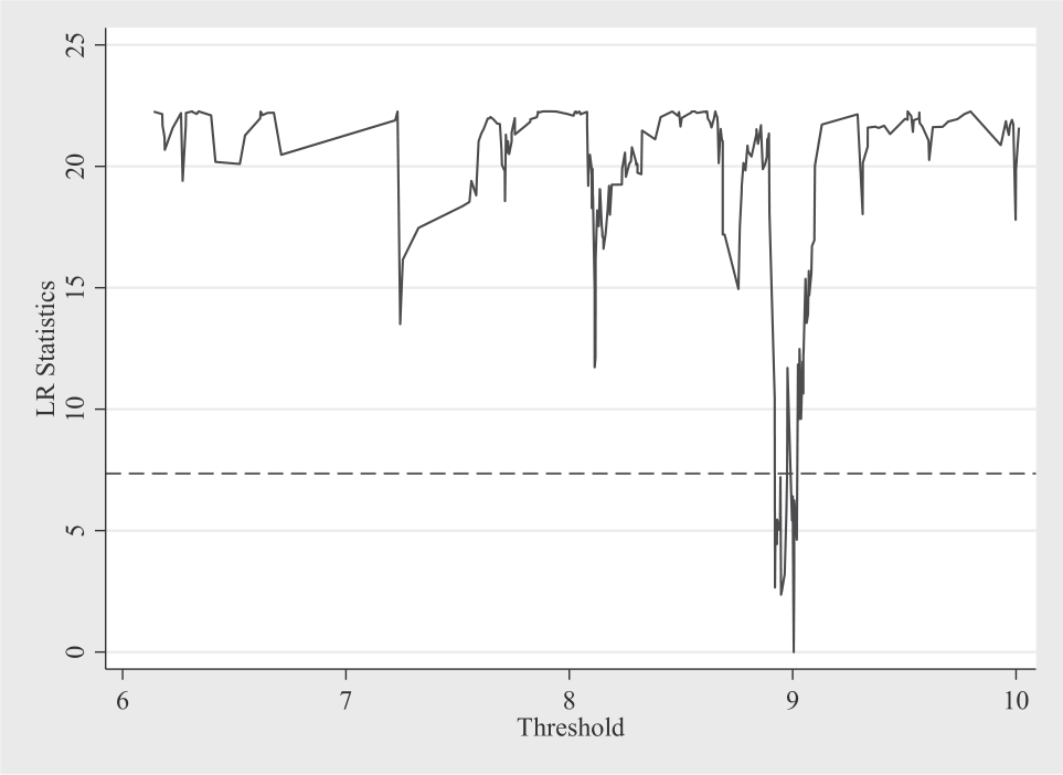
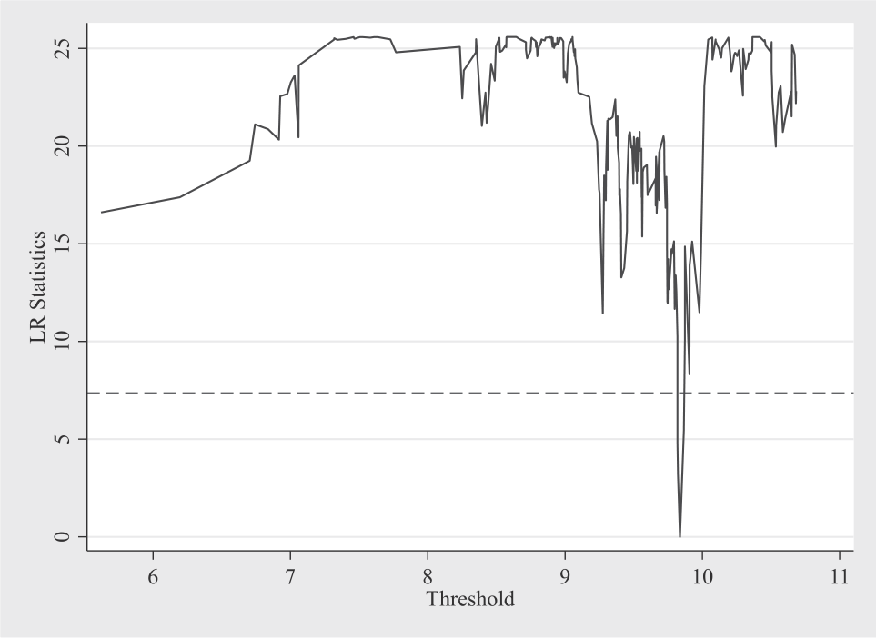
According to the multiple regression results above, this paper believes that there may be a nonlinear relationship in the mechanism of NUC’s impact on g2 and g4, so this paper decides to conduct further research based on threshold regression. Table 12 illustrates that there is a single threshold effect of NUC in the process of affecting Lnwastewater (g2) and Lnsmoke (g4). Regression (1) shows that when the regional secondary industry output value (Lngdpi2) is at a low stage, NUC has a significant weakening effect on industrial sewage discharge, and the result is significant at the 5% level. At this time, for every 0.1 unit increase in NUC, local industrial sewage discharge will decrease by 5.16%. When the output value of the secondary industry in the area is higher than the threshold, the impact of NUC on industrial wastewater is no longer significant. Regression (2) shows that when the regional coal consumption (Lnecc) is at a low stage, the impact of NUC on industrial dust emissions is not significant. When the coal consumption in the region exceeds a certain threshold, NUC will have a strong inhibitory effect on industrial dust, and the conclusion is established within the 1% confidence interval. In areas with higher coal consumption, every 0.1 unit increase in NUC will reduce industrial dust emissions by 21.3%. Fig. 16-17 shows the threshold regression chart, which proves that NUC does have a threshold effect on g2 and g4.

Fig. 16.

TR on Lngdpi2 for NUC.

Fig. 17.

TR on Lnecc for NUCs.

Conclusion and Policy Implications

Conclusion

The historical lessons of environmental disasters brought about by traditional infrastructure construction should not be forgotten. In the new era of China’s pursuit of high-quality economic development, the environmental disaster of infrastructure construction cannot be allowed to happen again. Although new infrastructure is considered green and low-carbon by many studies, unmatched new infrastructure investment still has the possibility of damaging the environment. Therefore, in the stage of the rapid growth of China’s new infrastructure investment, it is undoubtedly essential to prevent and control the pollution problems that may arise from mismatched new infrastructure construction.

Based on the above starting point, this study explores the potential impact of the matching degree of NII and UIS on environmental pollution from the perspective of coupling coordination between new infrastructure investment (NII) and industrial structure upgrading (UIS). Based on data from 30 provinces in China from 2011 to 2019, this paper constructs a new infrastructure investment index (NII) through the GPCA method. Then, the CCDM method is used to construct the coupling coordination index (NUC) of new infrastructure investment and industrial structure upgrading. In the part of the spatial effect, this paper uses the spatial autoregressive model to find that NII, NUC, PM2.5, and industrial sewage have positive spatial spillover effects, and there are “high-high” and “low-low” clustering characteristics. In the direct effect part, this paper uses the individual fixed effect model to find that NUC has a significant inhibitory effect on major environmental pollutants. In addition, the improvement effect of NUC on PM2.5 and industrial dust has a lag effect stronger than that of the current period. Among the direct effect results, only the effect of NUC on industrial wastewater discharge did not pass the multiple robustness tests of 2SLS and IV-GMM. In the indirect effect part, the study found that NUC can indirectly improve the environmental pollution level by promoting the energy consumption structure (ECS) and green innovation index (GII). The robustness test for the mediation effect also uses 2SLS and IV-GMM, where the regression results of NUC on industrial dust emissions through GII fail the robustness test. The mediation effect regression results and robustness test show that NUC increases the level of industrial sewage discharge by improving the energy consumption structure. However, NUC cannot improve the dust emission problem by improving the quality of green innovation. According to the direct and indirect effect results, this study believes that NUC may have a nonlinear effect on industrial sewage and dust discharge. The threshold regression results show that when the regional secondary industry output value (Lngdpi2) is at a low level, NUC significantly weakens industrial sewage discharge. Moreover, when Lngdpi2 is higher, the weakening effect of NUC on industrial sewage is not significant. Only when the coal consumption in the area exceeds a certain threshold for industrial dust emissions will NUC have a strong inhibitory effect on industrial dust. Otherwise, the results are insignificant.

Policy Implications

Based on the above research results, this paper provides the following policy recommendations:

1. Local governments should insist on promoting new infrastructure investment. In the post-epidemic era where economic recovery is slow, new infrastructure investment has a positive effect on the local economy and environment, and at the same time has its own spatial spillover effects, which are in line with the current macro requirements and realistic development needs of the green economy and low-carbon transformation. 2. The scale of local new infrastructure investment needs to match the local industrial structure. New infrastructure is a new driver to promote the upgrading of industrial structure, and unmatched new infrastructure investment choices will lead to waste of resources and environmental pollution. 3. Large industrialized provinces need to formulate special sewage control policies. The study found that sewage management in industrialized provinces cannot be solved through new infrastructure investment matching measures. On the contrary, a high matching level of new infrastructure investment will increase industrial sewage discharge. 4. Provinces with large coal consumption need to strengthen the matching degree between new infrastructure investment and industrial structure. The study found that for provinces and cities with large coal consumption, NUC will have a strong inhibitory effect on industrial dust, which will undoubtedly have a positive environmental improvement effect in areas with strong coal consumption demand.

6. Local governments must pursue long-termism in investing in new infrastructure. Since the environmental protection effect of NUC has a hysteresis effect and a threshold effect, local governments need to take a longer-term view of new infrastructure investment.

CONFLICT OF INTEREST

The authors declare no conflict of interest.

FOOTNOTES

1 The international environmental protection organization Greenpeace, the China Association for the Promotion of International NGO Cooperation, and the School of Environment of Renmin University of China jointly released “In-quiry into the Comprehensive Benefits of New Infrastructure Analysis Based on the Framework of Green and Inclusive Recovery”. Source: https://baijiahao.baidu.com/s?id=17161 87820096787632&wfr=spider&for=pc

2 Implementation in Stata. Source: Michael Stepner. (20l4). Binscatter: Binned Scatterplots in Stata. Slide deck online at https://michaelstepner.com/binscatter/binscatter-StataCon-ference2014.pdf.

3 Since the NII data has been standardized, the NII is represented here by the total amount of new infrastructure investment funds used by 10,000 people at the national level in Fig. 6. (Unit: Million CNY)

4 It should be noted that there are several macroeconomic variables among the explanatory variables in this study. Adding the time fixed effect at this time will produce multicollinear-ity, so this article uses the individual fixed effect model that reports the robust standard error for regression analysis. In order to test the robustness of individual fixed effects, this paper conducts tests based on 2SLS and IV-GMM respectively in the following part to check the reliability of the conclusions.

REFERENCES (41)

PAN J., ZHUANG G., ZHENG Y., ZHU S., XIE Q. Clarification of the Concept of a Low-carbon Economy and the Analysis of Its Core Elements. In Political Economy of China’s Climate Policy (pp. 179-198). Springer, Singapore. 2022.

Google Scholar

LIN B., ZHOU Y. Measuring the green economic growth in China: Influencing factors and policy perspectives. Energy. 241, 122518, 2022.

Google Scholar

ZHU S., HE C., LIU Y. Going green or going away: Environmental regulation, economic geography, and firms’ strategies in China’s pollution-intensive industries. Geoforum. 55, 53, 2014.

Google Scholar

YOUNG O.R., GUTTMAN D., QI Y., BACHUS K., BELIS D., CHENG H. (Eds.). Institutionalized governance processes: Comparing environmental problem solving in China and the United States. Global Environmental Change. 31, 163, 2015.

Google Scholar

ZHENG S., KAHN M.E. A new era of pollution progress in urban China? Journal of Economic Perspectives. 31 (1), 71, 2017.

Google Scholar

FENG Y., NING M., LEI Y., SUN Y., LIU W., WANG J. Defending blue sky in China: Effectiveness of the “Air Pollution Prevention and Control Action Plan” on air quality improvements from 2013 to 2017. Journal of environmental management. 252, 109603, 2019.

Google Scholar

ZENG Y., CAO Y., QIAO X., SEYLER B.C., TANG Y. Air pollution reduction in China: Recent success but great challenge for the future. Science of the Total Environment. 663, 329, 2019.

Google Scholar

GAO K., YUAN Y. The effect of innovation-driven development on pollution reduction: Empirical evidence from a quasi-natural experiment in China. Technological Forecasting and Social Change. 172, 121047, 2021.

Google Scholar

YANG X., ZHANG J., REN S., RAN Q. Can the new energy demonstration city policy reduce environmental pollution? Evidence from a quasi-natural experiment in China. Journal of Cleaner Production. 287, 125015, 2021.

Google Scholar

10.

GAO X., LIU N., HUA Y. Environmental Protection Tax Law on the synergy of pollution reduction and carbon reduction in China: Evidence from a panel data of 107 cities. Sustainable Production and Consumption. 33, 425, 2022.

Google Scholar

11.

LIU X., YANG M., NIE X. Can city brand reduce urban air pollution? An empirical research based on “National Civilized City” in China. Technological Forecasting and Social Change. 186, 122179, 2023.

Google Scholar

12.

WU T., SHAO W. How does digital economy drive industrial structure upgrading: An empirical study based on 249 prefecture-level cities in China. Plos one. 17 (11), e0277787, 2022.

Google Scholar

13.

ZHAO S., PENG D., WEN H., SONG H. Does the Digital Economy Promote Upgrading the Industrial Structure of Chinese Cities? Sustainability. 14 (16), 10235, 2022.

Google Scholar

14.

DOYLE M.W., HAVLICK D.G. Infrastructure and the environment. Annual Review of Environment and Resources. 34 (1), 349, 2009.

Google Scholar

15.

GUO K., PAN S. YAN S. New Infrastructure Investment and Structural Transformation. Chin Ind Econ. 03, 63, 2020.

Google Scholar

16.

DU X., ZHANG H., HAN Y. How Does New Infrastructure Investment Affect Economic Growth Quality? Empirical Evidence from China. Sustainability. 14 (6), 3511, 2022.

Google Scholar

17.

SU J., SU K., WANG S. Does the digital economy promote industrial structural upgrading? A test of mediating effects based on heterogeneous technological innovation. Sustainability. 13 (18), 10105, 2021.

Google Scholar

18.

XUE L., ZHANG Q., ZHANG X., LI, C. Can digital transformation promote green technology innovation? Sustainability 14 (12), 7497, 2022.

Google Scholar

19.

YU P., XU Z. The Impact of Digital New Infrastructure on the Green Technology Innovation Efficiency of Strategic Emerging Industries. Journal of Industrial Technological Economics. 01, 62, 2023.

Google Scholar

20.

ZOU T., GUO P., WU Q. Spatial and Temporal Evolutionary Characteristics and Driving Factors of Energy Green Consumption Levels in China: Based on the Perspective of Social Technology System Transition. Science and Technology Management Research. 22, 191, 2022.

Google Scholar

21.

ZHOU Y., CHEN J., ZHANG L., ZHANG Y., TENG C., HUANG X. Opportunity for Developing Ultra High Voltage Transmission Technology Under the Emission Peak, Carbon Neutrality and New Infrastructure. High Voltage Engineering. 07, 2396, 2021.

Google Scholar

22.

REN S., HAO Y., XU L., WU H., BA N. Digitalization, and energy: How does internet development affect China’s energy consumption? Energy Economics. 98, 105220, 2021.

Google Scholar

23.

LANGE S., POHL J., SANTARIUS T. Digitalization and energy consumption. Does ICT reduce energy demand? Ecological Economics. 176, 106760, 2020.

Google Scholar

24.

XU Q., ZHONG M., LI X. How does digitalization affect energy? International evidence. Energy Economics. 107, 105879, 2022.

Google Scholar

25.

ZHU B., ZHANG M., ZHOU Y., WANG P., SHENG J., HE K. (Eds.). Exploring the effect of industrial structure adjustment on interprovincial green development efficiency in China: A novel integrated approach. Energy Policy. 134, 110946, 2019.

Google Scholar

26.

HAN Y., ZHANG F., HUANG L., PENG K., WANG X. Does industrial upgrading promote eco-efficiency? ─ A panel space estimation based on Chinese evidence. Energy Policy. 154, 112286, 2021.

Google Scholar

27.

TIAN X., CHANG M., SHI F., Tanikawa, H. How does industrial structure change impact carbon dioxide emissions? A comparative analysis focusing on nine provincial regions in China. Environmental Science Policy. 37, pp. 243, 2014.

Google Scholar

28.

CHANG N. Changing industrial structure to reduce carbon dioxide emissions: a Chinese application. Journal of Cleaner Production. 103, pp. 40, 2015.

Google Scholar

29.

LI W., WANG W., WANG Y., QIN Y. Industrial structure, technological progress, and CO2 emissions in China: analysis based on the STIRPAT framework. Natural Hazards. 88 (3), 1545, 2017.

Google Scholar

30.

HAO Y., ZHENG S., ZHAO M., WU H., GUO Y., LI Y. Reexamining the relationships among urbanization, industrial structure, and environmental pollution in China – New evidence using the dynamic threshold panel model. Energy Reports. 06, 28, 2020,.

Google Scholar

31.

ZHU B., SHAN H. Impacts of industrial structures reconstructing on carbon emission and energy consumption: A case of Beijing. Journal of Cleaner Production. 245, 118916, 2020.

Google Scholar

32.

LI K., LIN B. The nonlinear impacts of industrial structure on China’s energy intensity. Energy. 69, 258, 2014.

Google Scholar

33.

FU H., MAO Y.S., SONG L.S. Empirical analysis on the effect of innovation on advancement of industrial structure process based on panel datas of provinces from 2000 to 2011. China Ind Econ. 09, 56, 2013.

Google Scholar

34.

SHENG K., SHI M. Promoting Industrial Transformation and Upgrading with New Infrastructure Construction. Journal of Jiangsu Administration Institute. 02, 42, 2021.

Google Scholar

35.

GONG X., LI D., ZHAO X. New infrastructure investment, industrial integration capacity and high-quality economic development. Price: Theory Practice. 04, 9, 2022.

Google Scholar

36.

ZHOU J., BAI Y. The Time Series’ Fluctuation and Regional Difference of the Urban-Rural Development Integration Level in China. China Industrial Economics. 02, 5, 2014.

Google Scholar

37.

LIU G. Global Principal Component Analysis of Competitiveness of China’s Regional Circulation Industry. China Economic Studies. 03, 79, 2014.

Google Scholar

38.

HOU Y., ZHANG K., ZHU Y., LIU W. Spatial and temporal differentiation and influencing factors of environmental governance performance in the Yangtze River Delta, China. Science of The Total Environment. 801, 149699, 2021.

Google Scholar

39.

DONG G., GE Y., ZHU W., QU Y., ZHANG W. Coupling coordination and spatiotemporal dynamic evolution between green urbanization and green finance: a case study in China. Frontiers in Environmental Science. 8, 621846, 2021.

Google Scholar

40.

LI J., SUN W., LI M., MENG L. Coupling coordination degree of production, living and ecological spaces and its influencing factors in the Yellow River Basin. Journal of cleaner production. 298, 126803, 2021.

Google Scholar

41.

HANSEN B.E. Threshold effects in non-dynamic panels: Estimation, testing, and inference. Journal of econometrics. 93 (2), 345, 1999.

Google Scholar

CITATIONS (1):

Rethinking energy allocation: Can green finance be the solution? — Evidence from machine learning method
Heyu Lu, Jiayang Li, Zongfa Wu, Yufeiyang Zeng
Energy

CrossRef

Submit your paper

Instructions for Authors

Publication Fees

eISSN:	2083-5906
ISSN:	1230-1485