

Introduction
With the growing global concern about atmospheric pollution, climate change, and quality of life, the reduction of greenhouse gas emissions has emerged as a pressing challenge. Among the major contributors to environmental degradation, road traffic transportation stands out due to its substantial impact on greenhouse gas emissions, congestion, and noise pollution. To tackle these issues, researchers have been actively exploring the application of green logistics and sustainable development concepts to curtail carbon emissions resulting from urban vehicle transportation. In this context, electric vehicles (EVs) have emerged as a promising solution to address environmental challenges and align with government planning objectives. However, EVs are not without their limitations, with restricted battery range and long charging times being particularly significant technical shortcomings. Consequently, the current implementation and applicability of electric vehicles are constrained. Given that the technical issues faced by EVs cannot be promptly resolved, the focus must shift towards devising strategies and optimization methods to mitigate carbon emissions and operational costs associated with transportation.
Compared with the Vehicle Routing Problem (VRP), the Electric Vehicle Routing Planning (EVRP) problem incorporates additional considerations, such as vehicle specifications, customer service time and location information, and the number of required recharges, owing to the limited range of electric vehicles. Furthermore, in addition to vehicle specifications, customer service time, and location information, the EVRP also addresses the number of charge cycles, charging strategy, and charging time due to the vehicle’s limited range. Research in the EV routing problem can be categorized into the following aspects: firstly, investigating the energy consumption patterns of EVs. Li’s study delves into the electric vehicle path problem, taking into account the constraints posed by battery life and battery replacement stations. The author starts by introducing an integrated model that incorporates factors such as speed, load, and distance to accurately measure the energy consumption and carbon emissions associated with electric vehicles [1]. Kim investigates the electric vehicle routing problem with nonlinear charging and discharging functions, where the rates of charging and discharging are state of charge dependent. The study explores the impact of state of charge related characteristics and proposes a nonlinear discharge function. In the distribution scenario, the vehicle’s cost is closely associated with its energy consumption, which, in turn, is influenced by the load size [2]. Pan addresses the issue of load variability and the stochastic nature of customer demand by proposing a model to solve the path problem for a vehicle with varying loads and uncertain demand [3]. He et al. investigated the impact of energy consumption on traffic congestion using an electric vehicle network equilibrium model [4]. Basso et al. presented a two-stage electric vehicle path problem aimed at enhancing the energy consumption estimation model that incorporates terrain and speed factors. The energy consumption of electric vehicles is influenced not only by the distance covered but also by various other factors, including effective load, speed profile (acceleration and braking patterns), road topography, instantaneous powertrain efficiency, and auxiliary equipment (e.g., air conditioner, refrigerator, etc.) [5]. The following aspect pertains to the electric vehicle charging strategy. Ge Xianlong et al. propose a flexible power replenishment strategy that takes into account both the remaining power of the vehicle and the number of remaining customers. This approach aims to ensure the efficient utilization of power resources [6]. Li Hao et al. developed a model incorporating charging queue time and charging time to investigate its influence on the equilibrium of a hybrid traffic road network [7]. Erdelic employed both single charging strategy and multiple charging strategy to compare and analyze their effectiveness in the EV path problem [8]. Afterward, Erdelic investigated both the partial charging strategy and the full charging strategy. By conducting a comprehensive comparison and analysis, it was found that the partial charging strategy leads to reduced waiting time and total trip duration. However, it comes with the trade-offs of increased driver’s psychological burden, a higher number of vehicles, and longer driving distances [9]. Li et al. proposed a wireless on the road charging technology, wherein vehicles are charged while driving. They developed a multi-objective path optimization model using model predictive control. This model aims to determine the most optimal path for drivers, considering both the wireless charging strategy and the plug-in charging strategy [10]. Froger et al. constructed a charging station with capacity limitations to address the EVRP model. They aimed to investigate the EVRP problem with a focus on nonlinear charging functions, multiple charging techniques, and en route charging with variable power [11]. In addition, there are EVRP that take into account various other factors. Keskin et al. introduced an EVRP variant with soft time windows and charging station waiting times. They divided the day into five time periods, each with different queue lengths, and employed an M/G/1 queuing system to calculate the waiting time at the charging stations for each time period [12]. Xiao et al. introduced a novel approach called the “Fixed Arc Detour Technique.” This technique involves incorporating a fixed optimal charging station access detour for each arc. Additionally, the authors devised a multifactor influenced electricity consumption model [13]. Zhang et al. utilized fuzzy numbers, grounded in reliability theory, to depict the uncertainty associated with service time, electricity consumption, and travel time [14]. Macrina et al. have introduced a novel GVRP (Green Vehicle Routing Problem) model tailored to a hybrid fleet comprising both electric and conventional vehicles [15]. In this study, Bac et al. tackled the local charging EVRP by considering multiple vehicle yards, heterogeneous electric vehicle fleets, and multiple customer visits [16]. Lin et al. examine the influence of time-varying electricity pricing on EVRP with time windows. They tackle the optimization of a multi-cycle vehicle path problem, focusing on electric vehicle charging and consumption scheduling schemes. The research sheds light on the effects of energy pricing, service hours, reduced winter range, and fleet size on EVRP solutions [17].
In recent years, numerous researchers have explored the integration of electric vehicles into the Cold Chain Vehicle Routing Planning (CVRP) problem. In CVRP, they endeavor to devise a driving speed profile that considers both congested and non-congested road traffic conditions [18]. Kok proposed a real road network speed model that accurately represents traffic congestion during peak hours. This model was subsequently applied to the cold chain VRP [19]. Based on this premise, Feng conducted a further investigation into the variation of vehicle speeds under various traffic congestion and weather conditions [20]. Poonthalir employed a triangular distribution to model the random travel speed, which represents the most probable speed between the maximum and minimum values [21]. In the context of EVRP, Zhao et al. presented a path optimization method for electric vehicles used in fresh food delivery, considering the impact of time-varying traffic conditions [22]. Currently, fresh food and other food products exhibit characteristics of being distributed in small and multi-batches within cities. In this context, the multi-temperature co-distribution model proves to be more suitable. This approach effectively addresses the challenge of uniformly delivering the demand for multiple layers in cold chain logistics while ensuring precise control of temperature and humidity to maintain product quality. Wang Shuyun et al. conducted a comparative study between two multi-temperature co-distribution modes: storage and mechanical. The comparison was based on various aspects, including their economic viability, safety, flexibility, and environmental impact [23]. Subsequently, they developed a mathematical model for storage multi-temperature co-distribution considering random demand scenarios. To address the challenges arising from random demand, an ex-ante estimation strategy was employed to solve the back-to-city replenishment problem [24].
In summary, in recent years, research on the comparative study of mechanical multi-temperature co-distribution, storage, and cooling, has predominantly centered around the application of conventional vehicles for distribution purposes. However, considering the unique requirements of urban fresh distribution and the pressing concern of air pollution, the distribution of goods using electric vehicles emerges as a promising and viable alternative. In previous literature, comparisons have been made between fuel vehicles and electric vehicles in logistics distribution. However, existing comparative studies have mainly focused on fuel vehicles, specifically those using storage and cooling type and mechanical type technologies. Unfortunately, there remains a research gap regarding storage and cooling type and mechanical type technologies under the context of electric vehicles. Most energy consumption models for electric vehicles typically focus solely on driving distance and often overlook the impact of load and other relevant factors. In urban road traffic scenarios, taking into account the time-varying road network environment can provide a more realistic representation of energy consumption and transportation costs. As a result, this paper aims to develop optimization models for the cold chain logistics path using both storage type and mechanical type electric vehicles. The objective is to minimize the total cost by considering the influence of load and speed variations on the energy consumption model within the context of the time-varying road network.
Problem Description
Research Hypotheses
The study assumes the presence of a single distribution center, an adequate number of electric vehicles available for distribution, and knowledge of the geographical locations of each customer point and charging station. Additionally, the demand, service time, and time window for each customer are known. Furthermore, the starting point of the vehicle is set to be the distribution center. The remaining assumptions are as follows:
(1) The electric vehicles operating under the multi-temperature co-distribution mode must adhere to the same specifications, and both the load and driving distance should not exceed the maximum limits defined by the vehicle specifications.
(2) The distribution process must not only meet the time window constraint but also adhere to the power constraint.
(3) When the electric vehicle’s power is insufficient to meet the distribution requirements, the vehicle needs to proceed to the nearest charging station for recharging. Charging is only deemed complete once the battery reaches its full capacity.
(4) The driving speed of the vehicle varies at different times of the day, and the average speed for each time period is known.
(5) The cold storage type of multi-temperature co-matching, utilizing thermal box transportation, provides enhanced product quality assurance, while also excluding cargo damage costs from consideration.
Research Questions: What are the distinctions between electric vehicle storage and mechanical transportation models? What are the comparative results for distribution costs? How does travel speed influence electric vehicle route selection? How does the energy consumption model, accounting for load and different speeds, impact the cost of the two distribution modes?
Symbol Description
M = {1,2,···,m} is the collection of the number of electric vehicles used. N = {0,1,2,···,n} is a distribution center with a collection of customer points. W = {0,1,···,w} is a collection of charging stations. Z = {1,2,···,z} is the set of transport product types. P11, P21 are the fixed costs per unit of ordinary electric vehicle and electric refrigerated vehicle, respectively. P12, P22 are the transportation costs per unit time for ordinary electric vehicles and electric refrigerated vehicles, respectively. P3 is the price per unit of electricity consumed. P4 is the charging price per unit of time. Ph is the unit price of product category h. P5 is the price per unit of product quality. Q, D are the maximum load and maximum driving distance of the electric vehicle, respectively. b is the maximum number of holding tanks per vehicle. aik, [Bi, Ei] are the arrival time of vehicle k at node i, and the time window of node i, respectively. xkij is the 0-1 variable, when the electric vehicle k is transported in i, j section, xkij = 1, otherwise xkij = 0. yjk is a 0-1 variable, electric vehicle k if it delivers for customer point j, yjk = 1, otherwise yjk = 0. zik is a 0-1 variable, zjk = 1 when EVk is charged at charging station i, otherwise zjk = 0.
Interventional studies involving animals or humans, and other studies that require ethical approval, must list the authority that provided approval and the corresponding ethical approval code.
Calculation of Travel Time Under Time-Varying Road Network
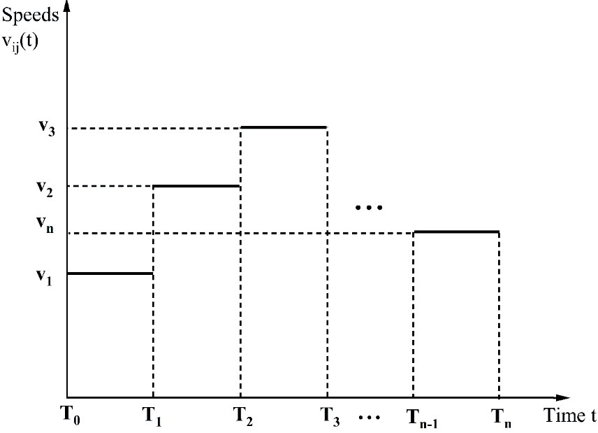
The speed within the urban road traffic network exhibits time variation. This means that the velocity of vehicles varies during different time periods, and the travel time for each road section between nodes is influenced by the starting point on that section and the remaining time within the current period. The average speed during each time period is depicted in Fig. 1. Classify the time of day as T = {[T0,T1],[T1,T2],···,[Tn-1,Tn]} ,The velocity changes in adjacent time periods. The velocities in each time period are V = {v1,v2,v3,···,vn},vn(t) is the average speed of travel at time t over time period [Tn-1,Tn]. dij is the distance of section [i,j]. The formula for calculating the travel time on section [i,j] is as follows.
Tij(0,ti+si) is the moment ti when the electric car arrives at the customer’s point i and serves the moment ti+si after Si time. Tij(ds,ts+ti+si) denotes the travelling time of the vehicle on the road section (i,j) from customer point i. ts is the time currently remaining in this time period, i.e., when t = [Tn-1,Tn], t = Tn˗t. ds is the distance traveled for the remaining time at the average speed for the time period in which it is currently located.
When ds<dij
When ds ≥ dij
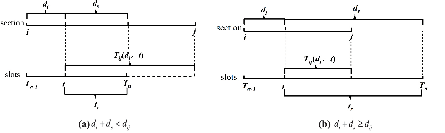
Tij(di,t) is the position on the road section [i,j] at time t, from i has traveled di distance, from this position to the customer point j time required to travel.
When di+ ds<dij
When di+ds≥dij
The theoretical diagram of section versus time for the above segmentation function is shown in Fig. 2. The formula is applied to the subsequent cost model to calculate the time required for different road sections.
Model Building
Cooling Storage Multi-Temperature Co-Mingling Model
Cold storage multi-temperature co-distribution involves utilizing room-temperature electric vehicles equipped with cold storage tanks for distribution. The total distribution cost comprises fixed costs, transport costs, holding tank expenses, and energy expenditures.
(1) Fixed and transport costs:
where K is the number of vehicles used. m is the number of available vehicles (k = 1,2,···,m). tijk is the travel time of EVk on the i, j sections.
(2) Cost of Insulation Boxes
where Ph is the unit cost of holding tanks for category h cold chain products. Nhk is the number of holding tanks used for loading category h cold chain products in the k th vehicle.
(3) Cost of energy consumption
The amount of energy consumed by electric vehicles is related to the load, speed, and transport time. In a time-varying road network environment, the electric power consumption of a vehicle traveling on the road sections i, j is:
Therefore, the energy cost of electric vehicles in the storage and cooling multi-temperature co-provisioning model is:
where P(Qk, v) is the operating power and g is the gravitational acceleration. A, Cd, and f are the wind-blown area of the EV, the air resistance coefficient, and the friction resistance coefficient of the car. ɳ is the mechanical transmission efficiency of the system. Q0 and Qk are the unloaded and current loaded weights of the EV.
(4) Cost of charging
When an electric vehicle’s remaining battery power is insufficient to meet the delivery requirements for reaching the next service point, it necessitates quick charging at the nearest charging station. The cost of charging is directly associated with the charging time.
The charging time is
where Emax is the maximum battery capacity of the EV. Eik is the amount of power left in the EV when it reaches the charging station, and rc is the charging efficiency of the charging station.
In summary, the total cost of the refrigerated multi-temperature co-mingling are
(11)
The constraints are as follows
(12) The results indicate that the number of distribution electric vehicles should be no less than the number of distribution routes. (13) It is required that a distribution center serves as the starting point for a vehicle to complete a distribution task. (14) Each demand point should be served by only one electric vehicle and served only once. (15) The total demand of customer points in each distribution path must not exceed the maximum capacity of the electric vehicle.
(16) The total distribution distance of each distribution path must not exceed the farthest distribution distance of the electric vehicle. (17) and (18) represent the time window constraints. (19) It is assumed that the EV leaves the charging station fully charged. (20) The constraint on the electric vehicle’s power to each customer point is denoted. (21) The number of holding tanks required is indicated.
Mechanical Multi-Temperature Co-Mingling Model
Mechanical multi-temperature co-distribution is accomplished through the utilization of electric refrigeration vehicles. The overall distribution cost primarily comprises fixed costs, transport costs, charging costs, energy consumption, refrigeration costs, and cargo damage costs. The computation methods for charging costs, fixed costs, and transport costs remain identical to those applied in cold storage multi-temperature co-distribution.
(1) Energy and cooling costs
Unlike cold storage distribution, mechanical multi-temperature co-distribution models incur electricity consumption during travel and energy costs for refrigeration trucks to provide refrigeration.
where Ec and Eo are the power consumption per unit of time during traveling, loading, and unloading, respectively. tik is the service time of the EV at customer point i.
(2) Cost of goods lost
The freshness of fresh products is related to the transport time; introducing the freshness of fresh products at
where ∂ is the cargo damage factor and qi is the demand at customer point i.
In summary, the total cost of mechanically co-mingling multiple temperatures is
(24)
The constraints are (12) to (20).
Algorithm Research
The solution of multi-temperature co-matching EVRP models using exact algorithms can be time-consuming. Therefore, heuristic algorithms are commonly employed to address these NP-hard problems. Among these, the genetic algorithm stands out as an efficient parallel search approach for tackling global optimization problems. The specific steps involved in applying the genetic algorithm to EVRP problems are as follows:
Step 1: Encoding and Decoding. In the context of the EVRP, the path selection process must take into account both the impact of the vehicle’s load and the necessity to visit a charging station when the electric vehicle’s power is low. To effectively represent the sequence in which each customer is visited in the instance, we employ a coding system using natural numbers to designate the customers. The customer numbers are represented as 1, 2,..., n. The distribution center is denoted as 0. Additionally, if there are m charging stations available, they are labeled as n+1,..., n+m. The first step involves arranging the customer nodes in ascending integer order, and then inserting the distribution center 0 among the customer points, considering constraints such as the vehicle’s maximum load and the demand at each node. Subsequently, the decision to visit the nearest charging station for recharging is based on the remaining power in the electric vehicle. If charging becomes necessary, the charging station number is inserted after the customer point number requiring recharging.
For example, consider an integer arrangement (6, 2, 5, 4, 3, 1, 7, 10, 9, 8) representing the customer point order. After incorporating the distribution center based on the load and time window constraints, the arrangement becomes (0, 6, 2, 5, 0, 4, 3, 1, 7, 0, 10, 9, 8, 0). Additionally, to cater to the electric vehicle’s low power situations, a charging station is inserted, resulting in the updated arrangement (0, 6, 2, 11, 5, 0, 4, 12, 3, 1, 7, 0, 10, 9, 8, 0). Decoding is the reverse process of encoding, wherein the decoded path for this chromosome is as follows:
Path 1: 0, 6, 2, 11, 5, 0
Path 2: 0, 4, 12, 3, 1, 7, 0
Path 3: 0, 10, 9, 8, 0
Table 1.
Customer location and demand information.
The study employs three electric vehicles for delivery purposes, each undergoing two charging events during their respective routes.
Step 2: Population initialization. The selection of the population size typically falls within the range of 20 to 200. If the number of chromosomes is too small, it may fail to yield the global optimal result. Conversely, an excessively large number of chromosomes will increase computation and impede solution efficiency. Consequently, we opt for a population size of 100.Each chromosome’s coding rule can be understood from the coding example in Step 1, where the customers are generated in random order. To create a single chromosome, we insert the distribution center and charging station based on load and power constraints. This process is repeated until 100 chromosomes are generated, thereby forming the initial solution.
Step 3: Determination of the adaptation function. The primary objective of both multi-temperature co-matching EVRP models is to minimize the total cost. In this context, the fitness value of the chromosome is directly proportional to the probability of its inheritance to the next generation. As a result, the fitness function is formulated as the inverse of the objective function.
Step 4: Selection. The selection process starts with an elite retention strategy, where fitness values are ranked based on their magnitude. The top 5% of chromosomes are preserved as elite candidates for the subsequent generation’s population. The remaining 95% of chromosomes are selected using the roulette wheel selection method. Chromosomes with high fitness are chosen for crossover and mutation in the next-generation population.
Step 5: Crossover. During the chromosome coding process in the EVRP problem, the insertion of charge station numbers may occur, and performing crossover and mutation can disrupt the original position of charge station insertion, resulting in numerous inferior solutions in the offspring. To address this, the gene representing the insertion of the charging station should be removed before carrying out the crossover and mutation operations. The crossover operation involves selecting genes that are not duplicated on the parent chromosomes and placing them sequentially into the offspring. For instance, considering parent P1 (1,2,3,4,5,6,7) and P2 (6,4,2,3,7,1,5), the crossover produces offspring O1 (1,6,2,4,3,5,7,1) and O2 (6,1,4,2,3,7,5).
Step 6: Mutation. Genetic variation is inherent in the process of genetic manipulation, and the mutation of chromosomes is necessary to avoid premature maturation, which could lead to rapid local convergence and ensure chromosomal diversity. To execute the mutation operation, several gene positions on the parent chromosomes are randomly selected and then rearranged, while keeping the other positions unchanged.
Step 7: Evolutionary Reversal Operation. In order to enhance the solution quality and expedite local convergence, a reversal operation is conducted on chromosomes that have already undergone selection and crossover mutation operations. The process involves randomly generating two integers to determine the positions within the chromosome, and subsequently reversing the sequence between the two positions, thereby generating a new chromosome. For instance, consider the parent chromosome P1 (1,2,3,4,5,6,7). Randomly generated integers, say 3 and 6, are used to perform the reversal operation, resulting in the offspring chromosome O1 (1,2,6,5,4,3,7). It is important to note that only reversals leading to improved fitness values are deemed valid.
Table 2.
Model parameter values.
| Parameter | Parameter value | Parameter | Parameter value |
|---|---|---|---|
| P11 | 100 yuan/veh | Q0 | 2t |
| P21 | 120 yuan/veh | g | 9.81 m/s2 |
| P12/P22 | 50 yuan/h | f | 0.015 |
| Ph | 15/25 yuan | Cd | 0.6 |
| P3 | 0.5 yuan/kwh | η | 1.46 |
| P4 | 1 yuan/min | Ec | 4kw/h |
| P5 | 1 yuan/kg | E0 | 5kw/h |
| ∂ | 0.01 | A | 6 m2 |
The number of iterations in the algorithm calculation is set to 500, and the calculation process will automatically terminate when this number is reached.
Example Analysis
Example Data and Parameter Setting
The experimental data is sourced from the Figshare database (https://doi.org/10.6084/m9.figshare.10288326), specifically utilizing the example R-2-C-30 as the simulation data. This particular example comprises 30 customer points and 2 charging stations. The coordinates of the distribution center are (43, 55), while the charging station coordinates are (25, 25) for station 31 and (50, 25) for station 32. To align with the necessary criteria, certain demand data are configured and presented in Table 1.
The speed of vehicles in urban road traffic varies with time, and these speeds are categorized into two periods: congestion and normal driving. The congestion period corresponds to the morning peak hours from 7:00 a.m. to 9:00 a.m., during which the average speed is 25 km/h. The normal driving period occurs during the evening peak hours from 5:00 p.m. to 8:00 p.m., with an average speed of 40 km/h.
The genetic algorithm was employed to address the problem using a computer processor with a clock speed of 2.20 GHz, 4 GB of memory, and MATLAB (R2018b). The relevant parameters were configured as indicated in Table 2.
Experimental Results Analysis
In this study, we employ the genetic algorithm to address the path optimization problem concerning storage-cooled multi-temperature co-distribution and mechanical multi-temperature co-distribution electric vehicles. The resulting vehicle transportation paths are presented in Table 3 and Table 4, while the path optimization diagram is depicted in Fig. 3.
From Table 3 and Table 4, it is evident that the number of distribution paths remains consistent in the optimal paths of the two multi-temperature co-distribution modes. In comparison to the refrigeration storage mode, the mechanical mode exhibits a more uniform vehicle load per path, higher charging frequency, and longer charging time. These differences can be primarily attributed to the mechanical multi-temperature co-distribution mode of electric refrigerated vehicles, which incurs power consumption during both driving and refrigeration processes. Considering electric vehicles with the same battery capacity, the storage and cooling method in multi-temperature co-dispensing transportation can effectively conserve energy and reduce resource wastage.
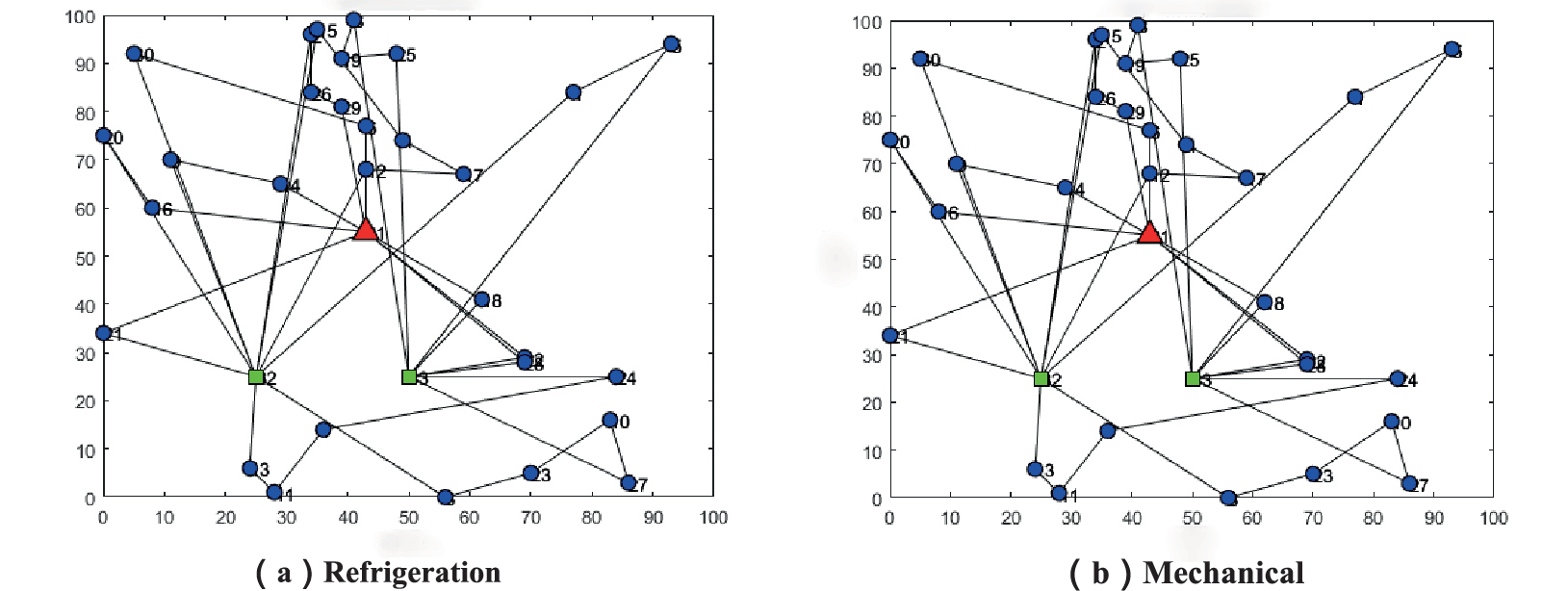
Table 3.
Accumulator type multi-temperature co-mingling path results.
| Number | Path | Load (kg) | Charging times | Charging time (h) |
|---|---|---|---|---|
| 1 | 0—29—16—9—20—31—13—7—23 –3—10—32—14--0 | 100 | 2 | 3.13 |
| 2 | 0—22—18—0 | 30 | 0 | 0 |
| 3 | 0—17—12—6—26—19—25—1—32—28—0 | 75 | 1 | 1.21 |
| 4 | 0—5—32—27—24—4—8—15—2—31—21—30—31—11—0 | 100 | 3 | 3.31 |
Table 4.
Mechanical multi-temperature co-mingling path results.
The experimental results for each cost are presented in Table 5. The table includes the following costs in yuan: fixed cost (GC), transportation cost (YC), energy consumption cost (NC), charging cost (CC), holding tank cost (BC), cargo loss cost (HC), and total cost (TC).
Based on Table 5, it is evident that:
(1) The total distribution cost of the cold storage type multi-temperature co-distribution is $375.99 lower than that of the mechanical type multi-temperature co-distribution, making it a more economically efficient option. Analyzing each cost component, the unit cost of mechanical multi-temperature co-distribution utilizing electric refrigerated cars is 50 yuan higher per car compared to ordinary electric cars. On the other hand, for the ordinary electric car’s storage type, insulation boxes are required to maintain the cold chain products’ freshness and meet the necessary temperature requirements. Consequently, an additional cost of 160 yuan is incurred for the insulation boxes. Considering both vehicle usage and preservation of freshness, the cold storage type proves to be 40 yuan cheaper than the mechanical type.
(2) The transportation cost of the mechanical type is $19.75 higher than that of the cold storage type. This cost discrepancy can mainly be attributed to the longer transportation time associated with the mechanical types. On the other hand, electric vehicles (EVs) incur additional energy consumption during the driving process, and the cooling of the freezer also adds to the electricity consumption. The energy cost of the EV’s driving process is dependent on factors such as speed, load, and delivery time, contributing to the mechanical type’s energy cost being as much as $201.27 higher than that of the storage and cooling type. As evident from Tables 3 and 4, the mechanical type also requires longer charging times, which further increases the charging cost.
(3) In comparison to cold storage type multi-temperature co-distribution, the utilization of mechanical electric refrigerated vehicles for distribution results in internal and external heat exchange during transportation and unloading. This leads to increased energy costs and cargo loss expenses. Moreover, besides ensuring product freshness, it facilitates the transfer of the insulation box and products to other suitable vehicles and allows for the reusability of the insulation box in case of transportation-related traffic congestion or accidents. As a result, the storage-type multi-temperature co-distribution transport mode offers enhanced economic viability, improved product security and safety, and higher resource utilization.
Sensitivity Analysis
(1) Battery Capacities Variation
The battery capacity of an electric vehicle significantly influences its range and charging time, consequently impacting the distribution path and cost. In this study, two multi-temperature co-distribution modes were considered, with battery capacities of 150 kWh, 120 kWh, and 100 kWh. The corresponding results and findings are presented in Table 6.
Table 5.
Distribution Cost Comparison.
| Distribution mode | Cooling storage type | Mechanical | Difference |
|---|---|---|---|
| GC | 400 | 600 | 200 |
| YC | 885.59 | 905.34 | 19.75 |
| NC | 147.78 | 349.05 | 201.27 |
| CC | 287.27 | 314.37 | 27.1 |
| BC | 160 | 0 | 160 |
| HC | 0 | 87.88 | 87.88 |
| TC | 1880.65 | 2256.64 | 375.99 |
Table 6.
Comparison of results for different battery capacities.
Table 7.
Comparison of results for different loads.
Table 8.
Comparison of different distribution results.
As shown in Table 6, the number of vehicles used remains constant for both modes, despite the variance in battery capacities. As the capacity decreases, so does the charging time. When the battery capacity is set at 100 kWh, the mechanical type exhibits the lowest energy and transportation costs, indicating lower power consumption and shorter transportation time. Moreover, the charging and cargo damage costs are also minimized, resulting in an overall optimal total cost at this battery capacity.
Due to the reduction in battery capacity, the charging frequency increases, while each charging time decreases. Consequently, there might be less remaining power after returning to the distribution center along the route. It is essential to avoid excessive unused power after a full charge. The storage and cooling-type multi-temperature co-distribution system, with a battery capacity of 120 kWh, exhibits a lower total distribution cost despite its higher charging cost compared to the 100 kWh battery capacity. Hence, for both distribution cost and power resource utilization, the storage and cooling-type system are optimized with a battery capacity of 120 kWh.
(2) Different loads
The results of the two multi-temperature co-matching modes with loadings of 100 kg, 80 kg, and 60 kg, respectively, are presented in Table 7.
From Table 7, it is evident that the maximum load capacity of the electric vehicle is 80 kg, while the conventional vehicle can carry up to 100 kg. The number of vehicles remains unchanged in both modes. Moreover, the costs associated with cargo damage and holding tanks show no significant variation. However, there is an increase in transportation costs and transportation time. Additionally, energy consumption costs and charging costs are higher. Notably, energy consumption costs are directly influenced by the load weight and transportation time. Despite the reduction in load capacity by 20 kg, there is a disproportionate increase in transportation time. Consequently, the energy consumption cost rises.
When considering a maximum load capacity of 60 kg for electric vehicles, it is evident that the existing fleet of electric vehicles cannot adequately meet the demand of each distribution point. Consequently, there is a need to increase the number of vehicles used, resulting in higher fixed and transportation costs. As a result, the overall distribution cost increases significantly. Hence, the selection of the vehicle’s load weight plays a crucial role in determining distribution costs, including energy consumption. Therefore, it is imperative to choose an appropriate electric vehicle loading capacity.
(3) Different speeds
In the congestion period, the speed cannot be controlled, while during normal driving times, there is room for speed control. The average speeds in the normal driving period are 40 km/h, 50 km/h, and 60 km/h, respectively. The corresponding solution results are presented in Table 8.
From Table 8, the relationship between speed, transportation time, transportation cost, and energy consumption cost becomes evident. As speed increases, both transportation time and transportation cost decrease, while the energy consumption cost increases accordingly. This observation holds true under the assumption of a constant load weight. The findings suggest that energy consumption is directly affected by the vehicle’s speed and transportation time. Consequently, selecting an appropriate driving speed can lead to electricity savings and a more efficient utilization of resources.
The lowest total cost of distribution for the cold storage multi-temperature co-distribution model occurs at a speed of 60 km/h. Despite the increase in energy costs, it does not fully offset the cost reduction achieved at higher speeds due to significant changes in transport costs. For the mechanical multi-temperature mode, the lowest total distribution cost is observed at a speed of 50 km/h. The variation in transport cost is relatively small when the speed is changed from 50 to 60 km/h. Additionally, the driving process incurs higher energy costs, and the refrigeration for freezing results in additional energy expenses, leading to considerable changes in energy cost and charging cost.
Consequently, to optimize economic efficiency, the normal driving speed is set at 60 km/h for the cold storage distribution mode and 50 km/h for the mechanical distribution mode. When the speed is set at 60 km/h, the total cost of the cold storage and multi-temperature co-distribution modes is minimized. However, as the speed increases, the transport cost varies significantly, and the increase in energy cost is insufficient to compensate for the reduced overall cost.
In the mechanical multi-temperature co-distribution model, the lowest total distribution cost is achieved at a speed of 50 km/h. The change in transport costs from 50 to 60 km/h is relatively small. Additionally, apart from incurring higher energy costs during travel, the reefer also generates additional energy costs during freezing. Therefore, to maximize economic benefits, the normal driving speed is set at 60 km/h for the cold storage distribution mode and 50 km/h for the mechanical distribution mode.
Conclusion
This study addresses the path optimization problem of cold storage multi-temperature co-distribution and mechanical multi-temperature co-distribution electric vehicles. The objective function is to minimize the total cost, and a genetic algorithm is utilized to solve the problem. Comparative analysis of experimental results reveals that the cold storage multi-temperature co-distribution mode offers higher economic benefits, safety, resource utilization rate, and applicability. The economic benefits mainly stem from lower total distribution costs. Safety and applicability are mainly attributed to the insulation box’s ability to maintain a constant temperature, ensuring product quality and food safety over the long term. In unexpected situations, such as traffic accidents causing severe road congestion during transportation, the insulation box can be easily transferred to other usable vehicles, demonstrating strong applicability. The reusability of the insulation box and the lower electricity consumption and charging requirements of electric vehicles in cold storage mode contribute to energy savings and efficient resource utilization.
Furthermore, we conducted a sensitivity analysis on the load capacity, maximum battery capacity, and normal driving speed of the two modes. The experimental results indicated that the cold storage multi-temperature co-distribution mode achieved the optimal total delivery cost when the battery capacity was 120 kWh, the maximum load capacity was 100 kg, and the normal driving speed was 60 km/h. On the other hand, the mechanical multi-temperature co-distribution mode attained the optimal total delivery cost when the battery capacity was 100 kWh, the maximum load was 100 kg, and the normal driving speed was 50 km/h.
It is essential to note that this study only focuses on the path optimization problem of multi-temperature co-distribution electric vehicles under predetermined demand. Future research could explore the integration of new technologies such as the Internet of Things and Big Data cloud computing to dynamically plan vehicle paths by updating demand data in real-time environments.

