

Introduction
With the increasingly serious problems of global environmental pollution and traffic congestion, electric vehicles are attracting attention as clean energy transport. The application of electric vehicles in the logistics industry has a broad prospect. With the improvement of environmental awareness and government support for clean energy, electric vehicles will gradually become the mainstream choice for logistics and distribution. Firstly, the zero tailpipe emissions and low noise characteristics of electric vehicles meet the environmental protection requirements of modern cities, helping to improve urban air quality and reduce noise pollution. Second, the operating cost of electric vehicles is relatively low, especially in long-term operations, which can significantly reduce fuel and maintenance costs, thus improving the profitability of enterprises [1]. In addition, with the continuous improvement of charging infrastructure and technological progress, the range and charging speed of electric vehicles will continue to improve. Further promoting its application in the field of logistics and distribution. However, a number of challenges need to be overcome to realize the widespread application of electric vehicles in the logistics industry. These include problems in charging infrastructure construction, charging technology innovation, and distribution path optimization [2]. One of the most prominent problems is the optimization of distribution paths. In the process of logistics and distribution, reasonable planning of the vehicle’s travel path not only improves distribution efficiency and reduces costs, but also reduces energy consumption and extends the range of electric vehicles. Considering the special characteristics of electric vehicles, including range limitations and uneven distribution of charging facilities, path optimization is crucial to achieving the effective application of electric vehicles in logistics and distribution.
The path optimization problem (EVRP) of electric vehicles in logistics and distribution is a topic of great interest. With the increase in environmental awareness and the development of clean energy, electric vehicles, as an environmentally friendly and efficient means of transport in logistics and distribution, have now been the subject of multidimensional research results. Chen [3] recently developed a set of cost-minimizing paths based on the operational information of networked electric vehicles, including energy consumption and travel time. Dastpak [4] considered allowing an electric vehicle to partially recharge its batteries. The charging time is modeled by a segmented linear charging function that relies on the technology that EVs can use to charge their batteries at public charging stations and is applied to the EVRP. Ginting [5] proposed a VRP optimization model for the EV path problem in order to find the best path choice to minimize the total cost of stationary vehicles, traffic, charging, battery replacement, and waiting. Wang [6] proposed a strategy to predict the queuing probability of EVs arriving at charging stations under the smart grid, and Yang [7] proposed an EV charging path optimization strategy under the “traffic price allocation” model for the current optimization problem of EV charging path planning. Facing the uncertainty of customer demand and dynamic traffic conditions, it becomes challenging to determine the optimal logistics and distribution routes under deterministic conditions. In order to solve this problem, some scholars have proposed a new approach to solving the single or multiple distribution center EV route optimization problem by using a robust optimization model [8, 9].
The study of charging strategy in the electric vehicle path optimization problem is an important topic in the current logistics and distribution field. With the wide application of electric vehicles and the increase in distribution demand, how to reasonably formulate the charging strategy to ensure the continuity and efficiency of electric vehicles in the distribution process has become an urgent problem. Chang [10] proposed a two-stage optimization method for the electric vehicle path problem with a hybrid charging strategy. In the first stage, a fuzzy transfer closure method is used to group customer orders, and in the second stage, decision variables and constraints related to charging strategies are introduced to establish a mixed-integer linear programming model considering the three charging strategies of fast charging. Elma [11] proposes a DC fast charging technology with a dynamic energy management system. Wang [12] introduces a dynamic vehicle path based on a hybrid charging strategy (Optimization Problem). Moghaddam [13] proposed a smart charging strategy that provides multiple charging options, including AC 2-stage charging, DC fast charging, and battery replacement facilities at charging stations. The synergy between electric vehicles and renewable energy sources can improve energy consumption and participate in grid regulation through vehicle-to-grid (V2G) technology. Jiang [14] proposed a hybrid charging strategy with adaptive current control in this synergistic process. To ensure the coordination between dynamic wireless charging mode electric vehicles and hybrid systems in microgrids, Zhou [15] proposed a synergistic strategy consisting of a two-layer control structure.
The energy consumption problem is a key consideration in the vehicle path optimization problem. Energy consumption not only directly affects the operating cost but also relates to the operational efficiency and environmental performance of the vehicle. The load capacity of a vehicle has a significant impact on energy consumption. A heavier load increases the resistance of the vehicle, which in turn increases the energy consumption. Zhang [16, 17] considered the energy consumption in the process of traveling on the road with refrigerated products in the process of cold chain logistics and distribution. A congestion avoidance strategy is used during vehicle road transport where dynamic load costs are considered. Ghobadi [18] proposed a new fuzzy two-stage vehicle path problem involving a heterogeneous fleet of electric and internal combustion engine vehicles (ICVs). The first echelon consists of recyclable waste collected from waste collection points and transported to the main centers by EVs. The second echelon is the transport of recyclable waste to the recycling centers via ICVs. In the proposed model, fuzzy numbers are used to represent the rate and energy consumption that depend on the amount of load, vehicle speed, and recyclable waste. Zhang [19] proposed a hybrid vehicle energy consumption prediction and control algorithm based on the minimum equivalent fuel consumption model. Sun [20] constructed an energy conservation equation for a mobile vehicle based on the principle of energy flow and elucidated the difference between it and the vehicle-specific power model. The optimal speed model based on the minimum spatio-temporal energy consumption is established by using the optimization principle, and the optimal speed is derived from the constraints of the road, vehicle, and environment.
In summary, research on EV distribution path optimization and charging strategies has made some progress. However, most of the researchers applied dynamic load factors to the EVRP problem with shallow analysis, which led to a large deviation between the optimization results obtained and the actual situation. And there are still many methods to be studied for charging strategies. The aim of this paper is to conduct an in-depth study on the distribution path and charging strategy of EVs by comprehensively considering the influence of dynamic loads, in which the charging strategy is analyzed in terms of whether or not it is fully charged versus fast and slow charging modes. It provides new ideas and methods to solve the problems faced by electric vehicles in the field of logistics and distribution and promotes the further development and application of electric vehicle technology.
Problem Description
Research Hypotheses
The study assumes the presence of a single distribution center, an adequate number of electric vehicles available for distribution, and knowledge of the geographical locations of each customer point and charging station. Additionally, the demand, service time, and time window for each customer are known. Furthermore, the starting point of the vehicle is set to be the distribution center. The remaining assumptions are as follows: (1) When the distribution vehicle leaves the distribution center, the battery is in a fully charged state. (2) Distribution vehicles only deliver a single type of goods. (3) The customer’s needs are met once in the distribution process. (4) The specifications of distribution vehicles are uniform. (5) Distribution vehicles can choose different charging strategies at charging stations. (6) The number of visits to each charging station is not limited. (7) Distribution vehicles need to return to the distribution center after completing the distribution task. (8) The entire distribution process is carried out without taking into account other special factors (such as traffic congestion, vehicle breakdowns, etc.), and the traveling speed is constant. (9) Distribution vehicles out of the distribution center from 0 time to start calculating. (10) The gradient of the road surface of each traveling route in the distribution network is 0.
(11) The service time of the distribution vehicle at each demand point is equal. (12) The power consumption rate of the distribution vehicle is affected by the amount of load and can be expressed by the load-consumption rate model.
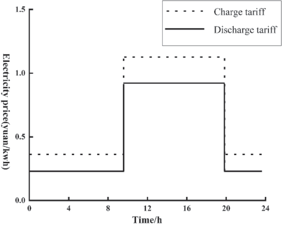
The tariff is a time-of-day, variable tariff, with different rates applied during different times of the 24- hour period. During peak hours, when the power system cannot meet the energy demand, the tariff is increased. Conversely, the price of electricity is reduced during off-peak hours. Fig. 1 presents the time-sharing tariff, derived based on distribution network load data from the literature [21].
Symbol Description
M = {1, 2, ..., m} is the set of the number of EVs used. N = {1, 2, ..., n} is the set of distribution centers and customer points. W = {n, n + 1, ..., n + m} is the set of m charging stations. Vk is the set of vehicle k traveling path nodes. qi is the demand of customer i. P1 is the fixed cost per unit of EV, P2 is the transportation cost per unit of time of EV, P3 is the price per unit of electricity consumption, Pi,t is the cost of charging per unit of power corrected for fast charging losses. Q, D denotes the maximum load and maximum distance of the electric vehicle, respectively. aik, [Bi, Ei] denotes the time of arrival of vehicle k at node i, and the time window of node i, respectively. E0 is the expected minimum charge during the driving of the electric vehicle. xijk denotes the 0-1 variable, xijk = 1 when electric vehicle k is transported in section i,j, otherwise xijk = 0. yik denotes the 0-1 variable, if the electric vehicle k delivers for customer point j, yik = 1, otherwise yik = 0. zik denotes the 0-1 variable, zik = 1 when EV k is charging and exchanging at i charging station, otherwise zik = 0.
Modelling the Relationship Between Load and Power Consumption Rate of Electric Vehicles
Within the field of pure electric vehicle distribution, the prevailing research does not consider the effect of cargo load weight on vehicle power consumption. When the vehicle load is different, the range of variation in fuel consumption of traditional internal combustion engines is small, while the battery power consumption of pure electric vans varies relatively more. Since the load of the vehicle changes as it passes through each customer point during the distribution process, the impact of the load of pure electric vehicles cannot be ignored. In this paper, we refer to the impact of cargo load on real-time power consumption of the vehicle as mentioned in the literature [22], and the formula is as follows:
Equation (1) represents the calculation of the vehicle power consumption rate under dynamic load. Pijk denotes the power consumption factor of vehicle k when traveling from node i to node j. Q0 is the vehicle weight. gr is the gravitational constant. ρ is the air density. A is the windward area. Cd is the aerodynamic drag coefficient. Cr is the rolling resistance coefficient. ε is the vehicle driveline efficiency. The specific parameter settings are shown in Table 1.
Charging Decision Model
To establish a charging decision model for EV distribution, the set of all nodes of EV is counted as N, and the behaviors in the EV distribution process are classified, and the classification indicator a can be expressed as [23]:
It has been shown that fast charging causes irreversible lifetime loss in EV batteries compared to slow charging, which causes negligible battery loss. Where the fast charging loss is modeled as:
Where: Qsite is the permanent reduction of battery capacity. Tacc is a constant related to temperature. Sacc is a constant related to battery capacity. cref, Dacc is a coefficient related to the rest of the battery’s own parameters. Nk is the number of charge/discharge times.
Neglecting the influence of the external ambient temperature, the battery loss mainly comes from the heating of the battery during charging, which is mainly caused by the high current generated by fast charging, and we can get the cost of the battery loss caused by a single fast charging:
Where: Closs is the main loss cost of the battery caused by a single fast charge. Qmax is the maximum capacity of the current battery. Q0 is the rated capacity. Ck is the cost of the battery per unit capacity. Tmax is the maximum number of cyclic charges, and the integral term is the fast-charging charging power. Pfast is the limiting fast-charging power. Ccharge is the charging power charged by the equivalent limiting fast-charging power. tstart, tend are the starting and terminating times of fast charging, respectively.
Table 1.
Energy consumption formula parameters.
| Parameter | Parameter value | Parameter | Parameter value |
|---|---|---|---|
| Q0 | 2000 kg | ρ | 1.293 kg/m3 |
| ν | 50 km/h | Cd | 0.30 |
| A | 3.6 m2 | Cr | 0.01 |
| gr | 9.8 | ε | 0.8 |
In order to improve time utilization, four charging strategies are considered to make charging decisions for the delivery service time interval. They are the charging model that gives priority to slow charging, the charging model that adds fast charging when slow charging does not satisfy the power balance condition, the path-planning fast charging model commonly used in existing research, the full charging strategy, and the incomplete charging strategy. That is, the charging quantity of electric vehicles during each charging in the distribution process is not necessarily the remaining capacity of the battery, but the decision is made according to the power consumption required for its subsequent services, which is explained as follows:
(1) Prioritise slow charging and shallow charging and discharging. The slow charging strategy is adopted under the condition that the sum of service hours is sufficient for slow charging to meet the power balance constraint. The charging nodes are selected according to the spatial and temporal distribution of electricity price and the principle of lowest electricity cost. the actual charging power ΔQi,chair of the EV at node i satisfies the constraint:
Where: yi,kslow is a 0-1 variable representing the slow charging decision, taking 1 for the slow charging condition only and 0 otherwise. ti,chair is the charging time at node i. Pchair,slow is the slow charging rate, respectively. M is the set of all EVs. ΔQchair is the theoretical charging amount, regardless of node.
If the full slow charging is not enough to offset the power loss required for the trip, the fastest possible fast charging strategy, i.e., fast-slow hybrid charging, is used. The appropriate fast and slow charging nodes are selected through the spatio-temporal distribution relation of electricity prices, which makes the electricity cost the lowest. The corresponding constraints are as follows: ∆Qi = Pchar slow i serve, t , yi kslow, + Pchar fast i serve, t , yi kfast, i ∈ N k, ∈ M (7)
Where: yi,kfast is a 0-1 variable representing the fast charging decision, taking 1 only for fast charging conditions and 0 otherwise. It is easy to know that under this charging decision, when yi,kslow is 0, it means that the charging station is not in the service opening time at the current time or fast charging is being carried out. Pchar,fast is the actual average fast charging power discounted by the stationing time, which ranges between slow charging and limit fast charging power.
(2) Fill-and-go. As a control strategy. The fast charging method is much higher than the slow charging method in terms of power, so the charging method on the way of distribution, i.e., under the power constraint, only a single fast charging is considered, while combining with the method of this paper to use the temporary parking time for charging. At this time, there is no need to consider the global constraint under satisfying the SOC instantaneous constraint, and the power level satisfies the following relationship:
(3) full charging incomplete charging. Different from the full charging strategy, under the incomplete charging strategy, the charging volume of electric vehicles in the distribution process is not the remaining capacity of the battery each time it is charged, but according to the power consumption required for its subsequent services to make a decision. Therefore, according to the actual distribution situation, the incomplete charging strategy model is as follows:
Where: dij is the distance from node i to node j. qik1 is the remaining charge of vehicle k when it reaches node i. tcj is the charging time of the vehicle at charging station j, j∈W. g is the battery charging coefficient. hik1 is the load of vehicle k entering customer node i, i∈W∪N. hik2 the load of vehicle k leaving customer node i, i∈Vk∪N.
Where: Eq. (10) represents the total amount of power required by vehicle k to serve the remaining nodes of the route after charging station j. Eq. (11) represents the charging amount when vehicle k travels from node i to charging station j for charging. Eq. (12) represents the charging time of the vehicle charging at charging station j. Eqs. (13) and (14) represent the constraints on the order of service nodes, i.e., i,l,m represent the order of serving customer nodes on the distribution path of vehicle k.
Model Building
(1) Fixed Costs and Transportation Costs
Where K is the number of vehicles used, m is the number of vehicles available (k = 1, 2, ..., m), and tijk is the travel k time of an electric vehicle in section i,j.
(2) Energy Costs
The energy consumption of electric vehicles is related to the load, speed, and transport time. In a time-varying road network environment. The power consumption of a vehicle traveling on road section [i,j] is Pijk.
Therefore, the energy cost of electric vehicles is
(3) Charging Costs under Different Charging Strategies
When the remaining power of the electric vehicle is not enough to complete the delivery requirements to the next service point, it needs to go to the nearest charging station for fast charging, and the charging cost is related to the charging time. The charging method is divided into fast and slow mixed charging and instant charging, of which fast charging will produce battery loss costs. This paper also proposes a complete and incomplete charging strategy. Among them, the charging cost under an incomplete charging strategy is:
Under the charging cost model, the following constraints need to be satisfied:
(23)
Where: Pijk is the driving energy consumption. zik is the charging decision variable, with charging counting as 1 and otherwise counting as 0. Qmin is the lower limit of power allowed in EV distribution, and Qmax is the maximum EV battery capacity. Constraint (18) indicates that the charging decision must occur within the charging station’s service range time, in which the change of power needs to satisfy constraints (19)-(21). Constraint equation (22) indicates that EV stop and wait does not consume power. Constraint Eq. (23) is the power consumption equation, where the 1st equation indicates the amount of slow charging and the 2nd equation indicates the amount of fast charging; Constraint Eq. (24) is the SOC inequality constraint for each moment.
The above are the constraints for the incomplete charging cost model, while the constraints under full charging need to be replaced for Eqs. (23) and (24) with the following constraints:
(4) V2G slow charging and discharging costs and battery wear and tear costs
Electric vehicles return to the distribution center after completing the distribution task. They can be charged and discharged at the distribution center at a slow rate according to the time-sharing tariff to obtain certain benefits. The cost of charging and discharging is
Where Pc and Pd denotes the charging tariff and discharging tariff, respectively. Wc and Wb denotes the charging and discharging power, respectively. a and b denotes the charging and discharging parameters, respectively. When charging, a is 1 and b is 0. When discharging, a is 0 and b is 1. T0 and T1 denotes the start time and end time of charging and discharging respectively. Electric vehicles are affected by ambient temperature, depth of discharge, number of cycles, and discharge power when discharging to the grid, and the impact on electric vehicle battery loss is not taken into account because of the use of a slow discharge mode in the distribution center, with a small charging and discharging power. The cost of battery loss mainly comes from the impact of deep discharge and ambient temperature change. Pb is the total price of the electric vehicle battery, and the battery loss cost is:
Where: ω is the temperature correction factor for the cycle life of a Li-ion battery at the given temperature T. φ can be defined as -0.795 as the depth of discharge correction factor for the cycle life of a Li-ion battery at any depth of discharge D. Ln represents the cycle life of Li-ion battery at standard conditions (D = 1). M represents the cycle life of a lithium-ion battery under standard conditions (D = 1).
(5) Penalty costs
The logistics distribution process should consider the customer’s satisfaction with the delivery time of the product. In terms of delivery, customers usually have certain limitations on delivery time. There is a soft time window and a hard time window. This model selects soft time windows for calculation according to the actual situation of urban distribution. That is, the customer requires delivery within [Bi, Ei] to describe the time window range. If delivered early, waiting costs are incurred. Penalty costs will be incurred if delivery is overdue. Therefore, the time penalty cost of this model is:
Where: θ1 is the cost factor for damaged goods delivered by delivery vehicles before the specified time in the time window. θ2 is the penalty cost coefficient for delivering vehicles beyond the specified delivery time window.
In summary, the total cost model of distribution, charging, and discharging in the electric vehicle switching mode is:
(30)
The constraints, except for (18-26), are as follows:
(31) denotes that the number of distribution electric vehicles is equal to or greater than the number of distribution routes. (32) indicates that the starting point of a vehicle to complete a distribution mission must be a distribution center. (33) indicates that each demand point can only be served by one electric vehicle, and only once. (34) indicates that the total demand of customer points in each distribution route must not exceed the maximum carrying capacity of electric vehicles.
(35) specifies that the total distribution distance of each distribution path shall not exceed the electric vehicle’s maximum distribution distance. (36) and (37) indicate the time window constraint.
Algorithm Research
The single distribution center multi-customer path optimization model constructed in this paper is a non-linear programming model that belongs to the NP-hard problem. Some precise algorithms in operations research can find the optimal solution for small-scale problems, and as the data size increases, the problem of “combinatorial explosion” occurs, while heuristic algorithms can get the approximate optimal results due to their stability and faster convergence, so this paper uses a genetic algorithm to solve the electric vehicle path optimization problem.
Step 1: Coding and Population Initialization. In genetic algorithms, all nodes are considered genes, and in this paper, the chromosome is formed by natural number coding, whose length is c + f + g +1. The code of the distribution center is 0; the code 1, 2, 3, ..., c represents the natural number sequence number assigned to each customer point; c + 1, c + 2, c + 1, c + 3, ..., c + f represents the natural number sequence number assigned to each charging station. A population is composed of a certain number of chromosomes, and in this paper, the following steps are to be followed to construct an initial population based on the carrying weight constraint:
(1) Randomize all nodes, including charging stations;
(2) qi denotes the distribution demand of customer node i, and qi' denotes the distribution demand of the customer corresponding to gene i in a chromosome.
If
(3) Repeat the calculation several times according to the above rule until the demand constraints of all customer points are processed;
(4) Form a complete initial chromosome by replacing 1 zero at the beginning and 1 zero at the end of the chromosome.
(5) Repeat the above operation to construct an initial population with population number N.
For example, a distribution center has a total of 3 electric vehicles serving 8 customer locations on a given day, and there are 2 charging stations in the distribution area. Assuming that a chromosome is formed after encoding: 0, 3, 6, 9, 2, 0, 1, 7, 0, 4, 10, 5, 8, and 0. Since each electric car starts from the distribution center and eventually returns to the distribution center, the split at “0” results in three routes, which can be interpreted as follows: the first car The first vehicle serves customer points 3, 6, and 2 in turn, and after leaving customer point 6, it drives to charging station 9 before serving customer 2; the second vehicle serves customer 1 and 7 in turn; the third vehicle serves customer 4, 5, and 8, and after leaving customer point 4, it drives to charging station 10 before serving customer 8.
Step 2: Determination of the adaptation function. The primary objective of both multi-temperature co-matching EVRP models is to minimize the total cost. In this context, the fitness value of the chromosome is directly proportional to the probability of its inheritance to the next generation. As a result, the fitness function is formulated as the inverse of the objective function.
Step 3: Selection. In this paper, instead of using selection operators, a certain proportion of individuals are selected. Firstly, the selection probability of each individual is calculated using the traditional roulette method and arranged in descending order; secondly, the first 1/3 of the chromosomes in the even-numbered positions are selected and retained for subsequent crossover operations; and finally, the new population is formed.
Step 4: Crossover. During the chromosome coding process in the EVRP problem, the insertion of charge station numbers may occur, and performing crossover and mutation can disrupt the original position of charge station insertion, resulting in numerous inferior solutions in the offspring. To address this, the gene representing the insertion of the charging station should be removed before carrying out the crossover and mutation operations. The crossover operation involves selecting genes that are not duplicated on the parent chromosomes and placing them sequentially in the offspring. For instance, considering parent P1 (1,2,3,4,5,6,7) and P2 (6,4,2,3,7,1,5), the crossover produces offspring O1 (1,6,2,4,3,5,7,1), and O2 (6,1,4,2,3,7,5).
Step 5: Mutation. Genetic variation is inherent in the process of genetic manipulation, and the mutation of chromosomes is necessary to avoid premature maturation, which could lead to rapid local convergence and ensure chromosomal diversity. To execute the mutation operation, several gene positions on the parent chromosomes are randomly selected and then rearranged while keeping the other positions unchanged.
Step 6: Evolutionary Reversal Operation. In order to enhance the solution quality and expedite local convergence, a reversal operation is conducted on chromosomes that have already undergone selection and crossover mutation operations. The process involves randomly generating two integers to determine the positions within the chromosome, and subsequently reversing the sequence between the two positions, thereby generating a new chromosome. For instance, consider the parent chromosome P1 (1,2,3,4,5,6,7). Randomly generated integers, say 3 and 6, are used to perform the reversal operation, resulting in the offspring chromosome O1 (1,2,6,5,4,3,7). It is important to note that only reversals leading to improved fitness values are deemed valid.
The number of iterations in the algorithm calculation is set to 500, and the calculation process will automatically terminate when this number is reached.
Example Analysis
Example Data and Parameter Setting
The experimental data is sourced from the Figshare database (https://doi.org/10.6084/m9.figshare.10288326), specifically utilizing the example R-2-C-30 as the simulation data. This particular example comprises 30 customer points and 2 charging stations. The coordinates of the distribution center are (43, 55), while the charging station coordinates are (25, 25) for station 31 and (50, 25) for station 32. To align with the necessary criteria, certain demand data are configured and presented in Table 2. The service time (i.e., temporary parking time) of the electric vehicle after arriving at each station is 90 min, and the initial time of departure is recorded as 0.
Table 2.
Model parameter values.
Table 3.
Time-sharing tariff.
| Types | Time period | Charge Price (yuan/kwh) | Discharge price (yuan/kwh) |
|---|---|---|---|
| Peak hours | 10:00-20:00 | 1.28 | 0.9 |
| Non-peak hours | 00:00-10:00 20:00-24:00 | 0.35 | 0.20 |
Electric vehicles complete their distribution tasks and return to the distribution center, where they are connected to the grid via batteries. Electricity is delivered to or obtained from the grid. sell electricity to the electricity market for a profit according to the impact of time-of-use tariffs. based on the time-of-use tariff data from the relevant literature [23], and to facilitate charging and discharging decisions. The day is divided into peak hours and off-peak hours, i.e., time-of-day tariffs, as shown in Table 3.
The genetic algorithm was employed to address the problem using a computer processor with a clock speed of 2.20 GHz, 4 GB of memory, and MATLAB (R2018b). The relevant parameters were configured as indicated in Table 2.
Experimental Results Analysis
In order to analyze the effectiveness of the proposed EV path planning and charging strategy model under dynamic load, four scenarios are set up for comparative analysis. Scenario 1 is that EVs are charged slowly with priority, then fast-charged according to the remaining distance and stopping time, and then leaving the charging station when the battery is full. Scenario 2 is EV charging on the go, i.e., fast charging and leaving the charging station with a full battery. Scenarios 3 and 4 are different from scenarios 1 and 2 in that they consider incomplete charging, i.e., charging the battery until it is enough to complete the remaining distance of the delivery and then leave the charging station. Using the genetic algorithm to solve the R-2-C-30 example under the four scenarios, the optimization path diagram of electric vehicle distribution is shown in Fig. 2, in which case the distribution paths of Scenario 1 and Scenario 3 and other related results are shown in Table 4.
As shown in Fig. 2, the number of EV crossover points is lower in Cases 3 and 4 with a fast charging strategy compared to Cases 1 and 2 with a fast and slow hybrid charging strategy. This leads to a reduction in charging time. The higher the number of crossing points, the longer the total logistics distribution path, which may lead to an increase in the distribution cost as well as a longer distribution time. Specifically, the charging time of EVs in transport with fast charging is longer than that with a fast-slow hybrid charging strategy. Since fast charging takes less time than fast-slow hybrid charging, i.e., the path crossing of the overall distribution will lead to an increase in the total transport time, the high economic efficiency of the distribution needs to be specifically analyzed based on the experimental results.
The experimental results of the specific paths with the number and time of charging for EV cases 1 and 3 are shown in Table 4. Both cases have the same number of charging times, but Case 1 has a longer charging time. That is, the charging time under the fast-slow hybrid charging strategy is about two times the charging time under the fast charging strategy. Although the charging time is slower, the distribution loads and paths of the four EVs in Case 3 are more evenly distributed, reflecting stability. The charging strategy in Case 1 has a relatively low impact on battery health.
The experimental results for each cost are presented in Table 5. The table includes the following costs in yuan: fixed cost (FC), transportation cost (TC), energy consumption cost (EC), charging cost (CC), V2G slow charging and discharging cost (VC), battery wear and tear costs (BC), penalty cost (PC), and total cost (TC).
Based on Table 5, it is evident that:
(1) The charging time of EVs under the fast and slow hybrid charging strategies is longer, but the charging cost is lower than under the fast charging strategy. The difference in charging cost between Case 1 and Case 3 is 100.36 yuan, and the difference in charging cost between Case 2 and Case 4 is 130.58 yuan. However, the relative increase in charging time increases the complexity of logistics and distribution. Case 1 and Case 2 have higher transport and penalty costs, i.e., lower service satisfaction at the point of demand. On the contrary, Cases 3 and 4 have higher battery wear and tear costs because the fast charging method has a greater impact on battery health, i.e., higher battery wear and tear costs. In case 4, compared to case 2, the energy consumption cost is higher by 78.75 yuan, but the transport cost is lower by 111.51 yuan. In terms of total transport and distribution costs, case 2 is more economical.
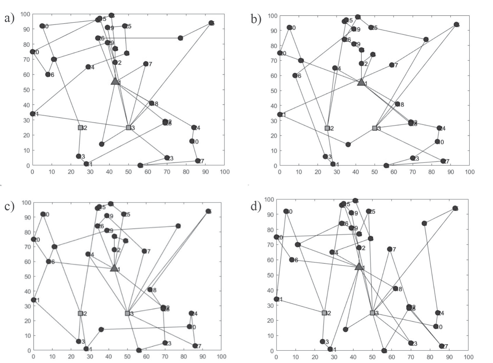
Table 4.
Driving records of vehicles
(2) Due to the constraints of vehicle loading and customer time window, the number of vehicles required from the two different charging strategies of Case 1 and Case 2 is the same, and the distribution paths are similar. Compared to the full charging strategy, Case 2 with the incomplete charging strategy has a shorter charging time and a shorter transport time, i.e., the charging cost is lower by 83.09 yuan and the transport cost is lower by 85.04 yuan. The saved delivery time correspondingly reduces the number of demand points that violate the customer’s time window constraints, which ultimately reduces the time window penalty cost and total delivery cost by 30.9% and 13.1%, respectively. It can be seen that when using electric vehicles for delivery, the incomplete charging strategy can not only save charging time and avoid the waste of vehicle residual power, but also reduce the total delivery cost while effectively improving customer time satisfaction.
(3) From the above four charging strategies, analyze the impact of slow charging and discharging management under consideration of V2G. For the complete charging strategy, slow charging and discharging can be based on time-sharing tariffs to obtain a certain amount of revenue and are conducive to the grid’s peak and valley value equalization. Since the charging amount under the incomplete charging strategy is just the amount of power arriving at the distribution center, there is no remaining power for charging and discharging management, but it is higher than the complete charging strategy in terms of charging time and customer satisfaction. Taken together, the total cost of EV distribution under the fast and slow mixed charging and incomplete charging strategies of Case 2 is the lowest and most economically efficient.
Table 5.
Distribution cost comparison.
Table 6.
Comparison of considering or not considering load impact.
Consider the Analysis of the Impact of the Load on the Path
This paper considers the influence of load on the real-time energy consumption of the vehicle and calculates the real-time energy consumption of the vehicle by establishing the energy consumption function of the power about the load weight to provide the basis for the path planning and charging strategy. The traditional energy consumption calculation method is to set a stable value. According to the actual parameters of pure electric trucks in China, the hourly power consumption of the vehicle is set to be 12. 5 kW at a speed of 50 km/h and a constant speed, which is combined with Case 1 in this paper to compare and analyze the path planning and charging strategy with or without considering the load. Table 6 shows the comparison of parameters between the two cases.
As shown in Table 6, there is no difference between Vehicle 1 and Vehicle 2 in terms of path planning and selection of charging station points, but Vehicle 1 has only 10.21% of remaining power when it goes to the nearest charging station 33 after completing the delivery task of Customer 3 without considering the effect of load, which will lead to overconsumption of power by the vehicle and may even cause the consequence of insufficient remaining power. Vehicles 3 and 4 change the choice of charging station without considering the effect of load, respectively, and the power is normal, but the total paths are increased by 6.51 km and 6.12 km. Therefore, considering the real-time effect of load on energy consumption facilitates the scheduling of appropriate charging plans and optimization in path planning.
Conclusions
In this study, the impact of dynamic loads on logistics and distribution is considered, and a relational equation between cargo loads and real-time vehicle power consumption is proposed and applied to the EV logistics and distribution path problem. At the charging management level, four charging strategies are designed in this study: fully charged or not, fast-slow hybrid charging, fast charging, and fully slow charging. These strategies are proposed with the aim of flexibly selecting the most appropriate charging method according to the real-time status of EVs, distribution demand, and fluctuations in electricity prices in order to maximize the economic benefits and reduce the pressure on the grid. The use of the fast-slow hybrid charging strategy is particularly critical. This strategy is used when the sum of service times is sufficient for slow charging to satisfy the power balance constraints, which ensures the power demand of EVs during the distribution process and takes full advantage of the lower battery loss from slow charging. When full slow charging is not enough to offset the power loss required for the trip, this study then uses a fast charging strategy with as little fast charging as possible in order to reduce the charging cost and the impact on the grid while ensuring distribution efficiency. In constructing the mathematical model, this study incorporates the application of different charging strategies with the objective of minimizing the total cost. The construction of this model enables us to consider multiple aspects such as transport cost, power consumption cost, charging cost, and battery depletion cost to derive the optimal combination of logistics and distribution paths and charging strategies. A genetic algorithm is used to solve the problem. The experimental results show that (1) the charging time under the fast-slow mixed charging strategy is about two times the charging time under the fast charging strategy. And it has a relatively low impact on battery health. Although the charging time is slower, the distribution loads and paths of the four EVs under the fast charging strategy are more evenly distributed, reflecting stability. (2) Compared with the full charging strategy, the incomplete charging strategy not only saves the charging time and avoids the waste of residual battery power, but also reduces the total delivery cost while effectively improving the customer’s time satisfaction.
(3) The total cost of EV delivery is the lowest and most economical under the mixed charging strategy of fast and slow charging. (4) Failure to consider dynamic loads can lead to excessive power consumption and may even result in insufficient residual power. Therefore, considering the real-time impact of load on energy consumption facilitates the scheduling of a suitable charging plan and can be optimized in route planning.
In future research, the selection of rechargeable customer points in the charging station selection strategy is a loaded research topic that can make the conclusions of this study richer and more effective. In addition to this, the research on EV delivery path optimization and charging strategies can be further improved by considering more load factors, introducing intelligent algorithms and machine learning methods, solving multi-objective optimization problems, and considering uncertainty.

