

Introduction
Climate change, a global phenomenon, has been at the forefront of scientific discourse due to its profound implications on both marine and freshwater environments [1-3]. These implications are not just limited to rising temperatures or altered precipitation patterns; they extend to the very fabric of aquatic ecosystems, influencing the dynamics of the marine food web and the organisms that constitute it.
Zooplankton, microscopic organisms that drift with ocean currents, play a pivotal role in marine ecosystems [1-3]. Serving as a crucial link in the pelagic food web, they connect primary producers, primarily phytoplankton, to higher trophic levels, such as fish. This intermediary role means that any change in the abundance, distribution, or community structure of zooplankton can have cascading effects on the entire marine food chain, ultimately influencing the dynamics of fisheries resources [1-3]. Given the economic and ecological importance of fisheries, understanding the factors that influence zooplankton dynamics is of paramount importance.
The seasonal variations in phytoplankton and zooplankton communities offer a lens through which we can observe the interplay of various ecological factors. These variations can serve as indicators of broader ecosystem changes, making them invaluable in the study of ecosystem dynamics. Moreover, they provide insights into the potential impacts of climate change on marine ecosystems [4-7]. As global temperatures rise and marine environments undergo transformation, the patterns of these seasonal variations might shift, potentially disrupting the balance of marine ecosystems.
Ecosystem models have emerged as powerful tools in the study of these dynamics. Over the years, researchers have applied these models to various oceanic regions, shedding light on complex interactions between physical and biological processes [8-12]. For instance, a three-dimensional circulation model has provided insights into water quality, touching upon aspects like nutrients, biochemical and oxygen demand, dissolved oxygen, and phytoplankton [13-15]. The choice of a model often hinges on the specific conditions of a region, the abundance of elements, and the accumulation of nitrate under different hydrodynamic conditions and seasons.
To provide a contextual backdrop for our study and to highlight the recent advancements in the field, a summary of pertinent recent research is presented in Table 1.
The Persian Gulf, particularly the Al Arish-Al Ghariyah coastal region of northern Qatar, presents a unique environment characterized by shallow depths and significant anthropogenic activities. Recent studies have employed remote sensing to understand the spatial and temporal variations of Chlorophyll-a (Chl-a) in these waters, a crucial indicator of phytoplankton abundance and primary production [4]. Such studies highlight the importance of regular Chl-a monitoring in marine waters, emphasizing the role of satellite data and specific algorithms in mapping Chl-a concentrations in arid regions [4].
The Gulf of Oman, an extension of the Arabian Sea, is a region of particular interest in this context. Positioned between Iran, Oman, and the United Arab Emirates, it serves as a gateway to the Persian Gulf from the Arabian Sea and the Indian Ocean. This marine region is not just geographically significant; it’s ecologically vital as well [16-18]. The Gulf of Oman is a major marine fishery production area, teeming with marine life and biodiversity. However, it’s also a region in flux, undergoing structural and functional changes due to a combination of climate change and anthropogenic activities [19-21]. The hydrodynamics of this region are intricate, influenced by a myriad of processes, including biogeochemical processes typical of upwelling, oligotrophic, and low-oxygen environments [22-24].
The Gulf of Oman experiences pronounced atmospheric forcing during the southwest monsoon (from late May to September) and the Northeast monsoon (from December to March). These monsoons introduce significant seasonal variability in biological productivity [25-27]. Such variability, driven by physical conditions like surface light, water temperature, and the depth of the upper mixed layer, can influence the cycle of plankton populations in the region [28].
Table 1.
Summary of recent studies on marine ecosystem modeling and their key findings.
Recent studies have delved into the biological and chemical parameters of the Persian Gulf and Oman Sea, employing coupled physical-biological ROMS models and satellite data to explore various facets of marine ecology [24-29]. However, there remains a gap in our understanding of the behavior of biological parameters with seasonal changes in the Oman Sea region, especially in the context of basin hydrodynamics and atmospheric forces.
In light of the above, the present research couples the Regional Ocean Model System (ROMS) with a biological model to simulate plankton groups in the Oman Sea. This model incorporates physical components to simulate ocean hydrodynamics and biogeochemical modules like BioFennel, Ecosim, Nemuro, NPZD-Franks, NPZD-Iron, and NPZD-Powell to simulate the evolution of biological components. The study aims to describe the seasonal patterns in growth limitation for phytoplankton and zooplankton and to evaluate the intertwined role of physical and biological processes as drivers of plankton seasonality in the region.
Materials and Methods
A coupled physical-biological ROMS model was used to predict seasonal changes of some biological parameters over the Persian Gulf and Oman Sea due to physical forces. ROMS is a new-generation ocean circulation model that is specially planned for accurate simulations of regional oceanic systems [34]. It is a split-explicit, free-surface ocean model, where short time steps are used to advance the surface elevation and barotropic momentum, with a much larger time step used for temperature, salinity, and baroclinic momentum. This model can solve Reynolds-averaged Navier–Stokes equations using hydrostatic and Boussinesq assumptions, in Cartesian coordinates on the horizontal, and sigma coordinates in the vertical direction. The model offers various ecosystem sub-models for ecological complexities [35].
NPZD is a nitrogen-based model which includes six variables: Ammonium (NH4), Nitrate (NO3), Phytoplankton (P), Zooplankton (Z), and large and small detritus (D) [36]. The schematic of the NPZD model is presented in Fig. 1.
The four dynamical equations have the same form. The left-hand side of each equation contains two terms: a local time derivative, and an advective term. The right-hand side includes biological dynamics except for the last term which is vertical mixing. The four dynamical equations have the same form. The left-hand side of each equation contains two terms: a local time derivative, and an advective term. The right-hand side includes biological dynamics except for the last term which is vertical mixing [37].
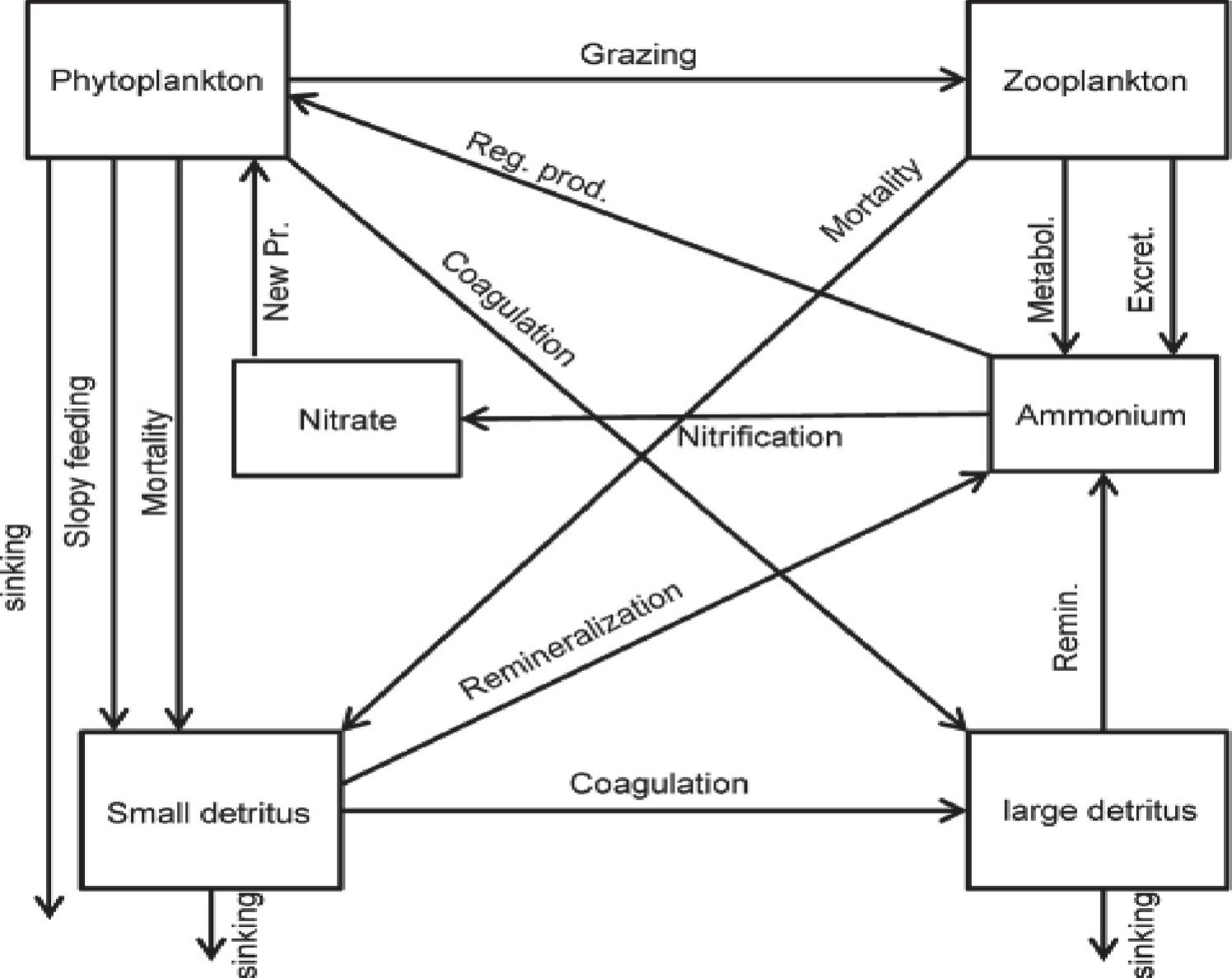
Major proceedings in this model include photosynthetic growth and uptake of nitrogen by phytoplankton (U), grazing on phytoplankton by zooplankton (G), mortality of both types of plankton for phytoplankton and zooplankton, and sinking and re-mineralization of detritus. Where diurnally and seasonally varying solar radiation (W.m-2) at depth z, is the incoming solar radiation at the water surface (Wm-2). The parameters used in the model are listed in Table 1.
The growth rate of phytoplankton depends on temperature and will be a function of the amount of photosynthetically active radiation, which, in turn, is a function of the time of the year, latitude, mixed layer depth, the light absorption properties of the water column, the characteristics of the phytoplankton photosynthesis-irradiance relationship and the nature of the nutrient limitation of cell growth [38]. The temperature’s function is based on the Arrhenius equation [39]. Light attenuation with depth is modeled using the Beer Law [40].
In modeling zooplankton dynamics, accuracy is important because zooplankton can have a critical impact on several environmental issues ranging from eutrophication to climate change. As zooplankton are among the most abundant creatures in the ocean and can easily absorb carbon, they can potentially combat global climate change. Zooplanktons are also the primary food source for many species of fish and are therefore indicator species. Any significant decline in zooplankton populations could negatively impact other species including endangered ones. Because of zooplankton’s importance in marine ecosystems, there is a clear need to be able to come up with accurate mathematical mortality rates [41]. Detritus is added to the water column through non-predatory phytoplankton and zooplankton mortality. Ammonium is generated through the mineralization of DN, the immediate mineralization of fractions of phytoplankton death, and zooplankton excretion. Nitrification is the biological oxidation of ammonia or ammonium to nitrite followed by the oxidation of nitrite. The transformation of ammonia to nitrite is usually the rate-limiting step of nitrification. In the ocean, nitrogen is often the limiting nutrient, so the nitrogen cycle is of particular interest because it creates nitrate, the primary form of nitrogen responsible for production. Nitrification is formally a two-step process: in the first step, ammonia (NH3) is oxidized into nitrite (NO2-); and in the second, nitrite is oxidized to nitrate (NO3) [42].
The model domain embraces the Persian Gulf and the Gulf of Oman. Nesting of the Persian Gulf within the Oman Sea allows us to explain circulation and variability in the Oman Sea domain. The open boundary was given in east, and the Flather method was used for barotropic velocities and mass conservation enforcement. The horizontal resolution of the model was extracted from ETOPO1 (Earth Topography 1 arcmin) with a 4-km resolution. Vertical distribution is made up of 30 terrain-following sigma layers to resolve surface and bottom boundary layers.
Furthermore, the spatial resolution of the model is 1/20 and the time step is 300 s. The initial conditions for temperature, salinity, nutrients were extracted from World Ocean Atlas 2009 (WOA2009). WOA9 is a collection of long-term data of temperature, salinity, oxygen, nitrate, silicates and phosphates for annual, seasonal and monthly periods for the world’s oceans. The NCEP meteorological data sets (reanalysis atmospheric model) are applied every 6 hours by computing different atmospheric parameters such as surface forces, surface wind stress, surface heat, cloud cover percentage, latent heat, relative humidity, surface pressure, average speed and direction of monthly wind. Also, we used SeaWiFS data for surface chlorophyll climatology dataset. To compare the results of the model with satellite data, global surface chlorophyll with accuracy of 4 km resolution was obtained from GMIS archive and after performing some corrections values for the study region were extracted and used.
The model was forced using the atmospheric forcing fields based on monthly climatology derived from the comprehensive Ocean-Atmosphere Dataset (COADS) [43]. In present paper, The ROMS-NPZD coupled system, is forced by climatologically atmospheric data and predicts the physical variables and concentrations of nitrate, phytoplankton, zooplankton, and detritus from 2006-2012 and finally results of 2008 were used for analysis.
To estimate the differences between modeled chlorophyll-concentrations and those of satellite-derived data, the results for several methods are used to evaluate the performance of the NPZD model in predicting the chlorophyll-concentrations. These include the standard deviation (SD) of the variability of chlorophyll-a, Pearson correlation coefficient (r) and the root mean square (RMS). We attempt to evaluate the monthly variability by computing the following standard deviation:
Where xi and yi represent the monthly and the annually averaged chlorophyll-a concentrations, respectively. The root mean square was used to illustrate the similarities and differences between the three areas.
Results and Discussion
Chlorophyll Distribution and Seasonal Variability
To assess the ability of the coupled ROMS-NPZD model over Gulf of Oman along with a cross-section (DE path as shown in Fig. 2) the distribution of chlorophyll was compared for winter and summer (Fig. 3). To display temporal changes of biological parameters, the time series at three selective points located at north-west (point A), south-west (point B) and north-east of Oman Gulf (point C) are illustrated. The maximum Chl-a concentration was observed in winter while the minimum was in summer. The highest Chl-a concentrations were observed in coastal areas with an average of 1.5 to 2 mgClm−3 in January and the lowest average of 0.5 to 1.0 mgClm−3 in the northern part of Oman Gulf. In these regions, maximal chlorophyll concentrations were observed during the winter monsoon (January-March). Geographic locations of the points are shown in Fig. 2, According to mean monthly patterns and time series of surface chlorophyll changes (Fig. 3) it is forecasted that the two regions can be separated based on the amount of surface chlorophyll. In September, the concentration of chlorophylls extends along the southern coasts of Oman sea, and then it was carried to the north of Oman sea and the coasts of Strait of Hormuz through the currents caused by meso-scale eddies. In January, the density of chlorophylls increased and covered major parts of the northern areas of the Persian Gulf and the Strait of Hormuz and the northern and southern regions of the Oman Sea. The average chlorophyll concentration in January in Oman Sea was higher than the Persian Gulf.
Fig. 3 also shows a large difference in maximum amount of chlorophyll in location A and C locations (around 1 and 2 mgClm−3 respectively), compared to location B (around 0.5 mgClm−3) and their temporal peaks in northwest occur in early winter, and for northeast regions in late summer.
Vertical Distribution of Chlorophyll-a
Vertical distribution was selected to display the concentration of chlorophyll-a during winter and summer on the north coast. During winter, model show maximum chlorophyll of 2 to 2.5 mgClm-3 in the upper 50 m depth of the water column along the coast. In lower depths, chlorophyll concentration decreases to between 0.75 to 1 mgClm-3. Along the same latitude, a moderate maximum of subsurface chlorophyll was observed occurring in January (Fig. 4). During summer, model display minimum chlorophyll of 0.5 to 1 mgClm-3 in the upper layer, and then it decreases at lower depths to 0.1-0.3 mgClm-3. Monsoonal and regional winds play an important role in regulating algal blooms. In general, the wind-induced mixing of the upper layer is mostly associated with wind stress than wind speed; however, both are important. During winter due to presence of anticyclones eddies (as can be seen in Fig. 8), there is an increase in chlorophyll where anticyclonic eddies cause water particles to pump upwards. During summer due to weaking of the eddies and chlorophyll concentration rapidly decreases.
Fig. 2.
Geographical location of Persian Gulf and Oman Sea; and A, B and C points located in 56.8°E-25.5°N, 59.9°E-24.3°N and 60.3°E-25.2°N respectively; and vertical cross-section along DE line from 57.5°E, 25.3°N to 59.5°E, 24.6°N.
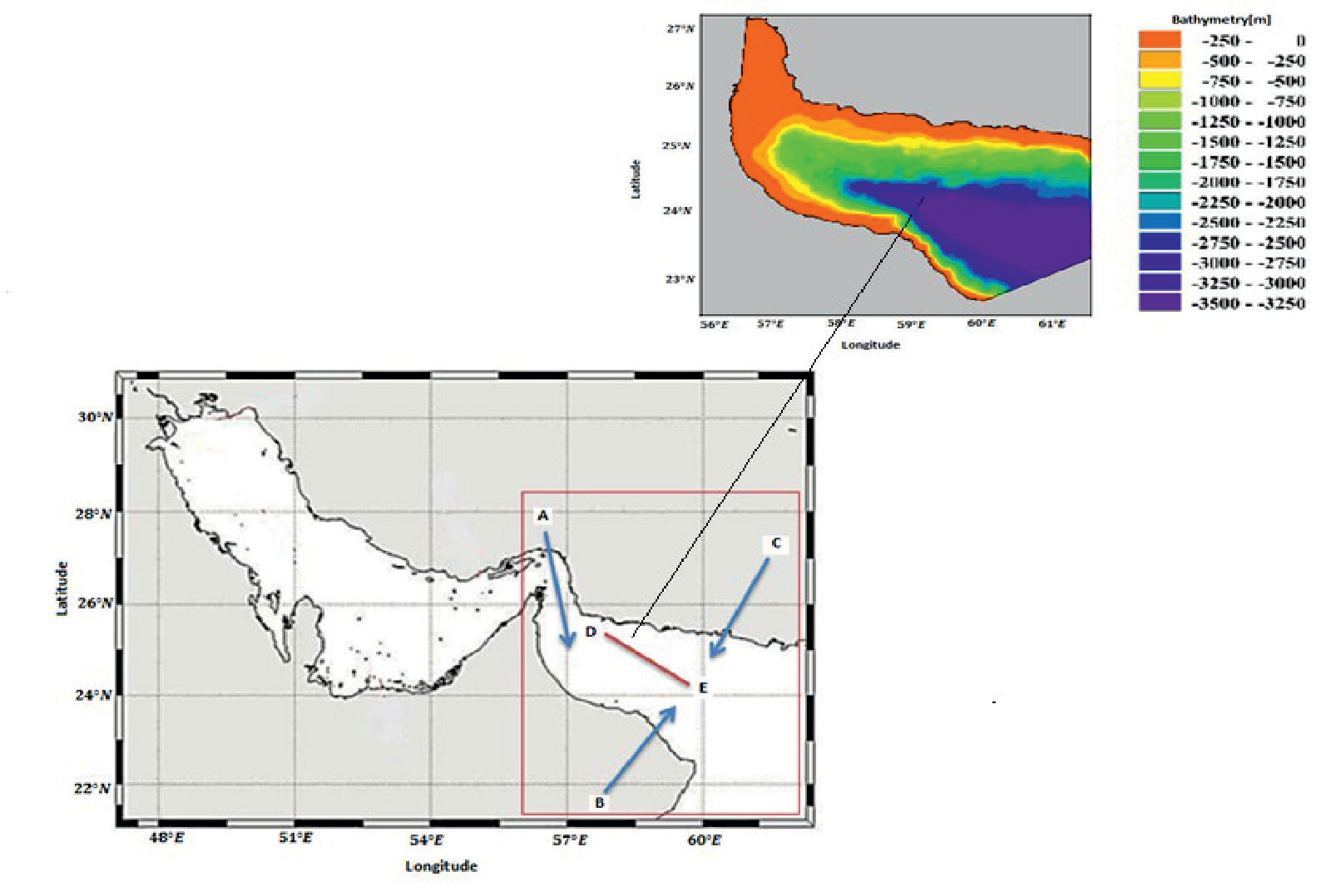
Fig. 3.
Mean monthly surface chlorophyll concentrations in Persian Gulf and Sea of Oman in January and July.
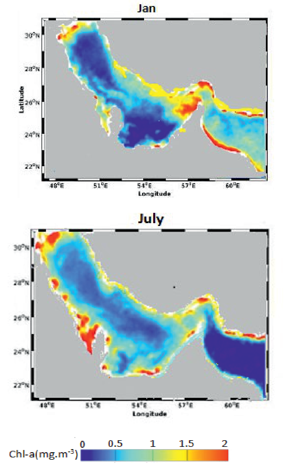
Fig. 5.
Monthly chlorophyll time series from the NPZD-ROMS model and SeaWiFs in Areas A, B and C (2008).
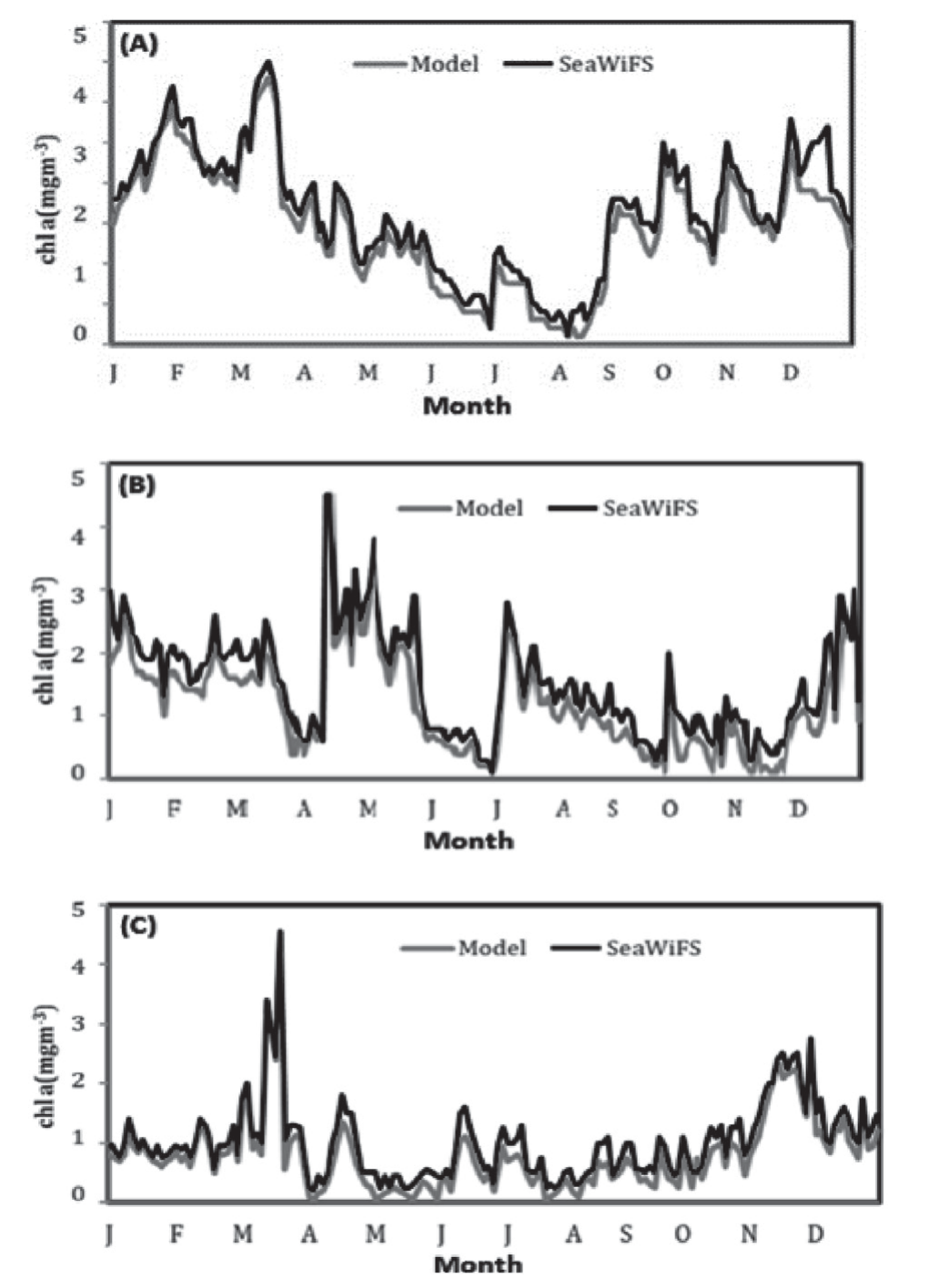
To compare seasonal climatology from model Outputs and satellite observations, we derived monthly time series of chlorophyll (Fig. 5) in three regions between 56.8°E to 59.9°E (Fig. 2). In the time series of chlorophyll-concentrations, in Areas (A) and (B), maximum values are reached in March and April, respectively. In addition, the lowest levels are reached in August and October to December, respectively. In Area (C), maximum level is reached in late winter and minimum in August to September. In Areas A and B, the chlorophyll-a concentration showed two marked maxima: one in winter and one in late autumn. A and B areas are the two productive regions, strongly influenced by the upwelled water flows northward and affect the oceanic stratification of the Gulf of Oman through gyres and eddy systems that sweep into the Oman Sea. The SW monsoon is also a major climatic factor affecting the near-shore environment and areas of coral growth in the Oman Sea during the summer months. Circulation in the Gulf of Oman is dominated by a cyclonic eddy in the west and an anticyclonic eddy in the east. The simulated chlorophyll time series are fairly correlated with the satellite chlorophyll-a time series. The modeled chlorophyll-a was at its peak during late winter (3.5 mgClm-3) and at its lowest during summer (0.2 mgClm-3). Time series of both remain with relatively high concentrations during winter and low concentrations during summer (Fig. 5).
Fig. 4.
Vertical chlorophyll concentrations in the DE cross-section in January and July, respectively.
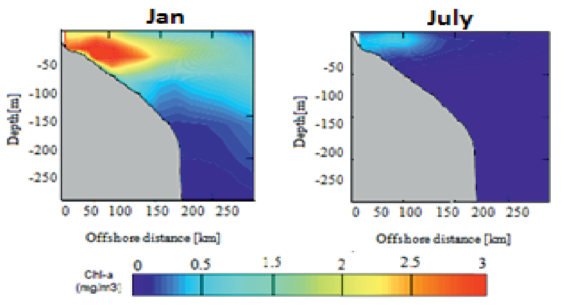
The simulated results are generally aligned well with the SeaWiFS observations with the correlation coefficient ranging from 0.968 to 0.985 and standard deviation from 0.814 to 1.26. There was a significant positive correlation between the chlorophyll-a concentration of the modeled data and satellite data (p<0.0001) (Tables 2 and 3). The smaller RMSE value represents higher accuracy in Area A.
Temperature Profiles and Seasonal Variations
Seasonal vertical distribution of temperature, which has been selected for the present study, shows the seasonal changes of the sea surface temperature. On average, SST ranged between 20 and 35 with the maximum value during summer and a minimum in winter between 22.5 and 25ºC. The low temperature in the surface water can be determined accurately and it can be about 2 to 3ºC lower than the offshore water (Fig. 6). The lowest water temperature in the Oman region is reached during winter months which is not only because of the latitude but also the retreat in monsoonal currents.
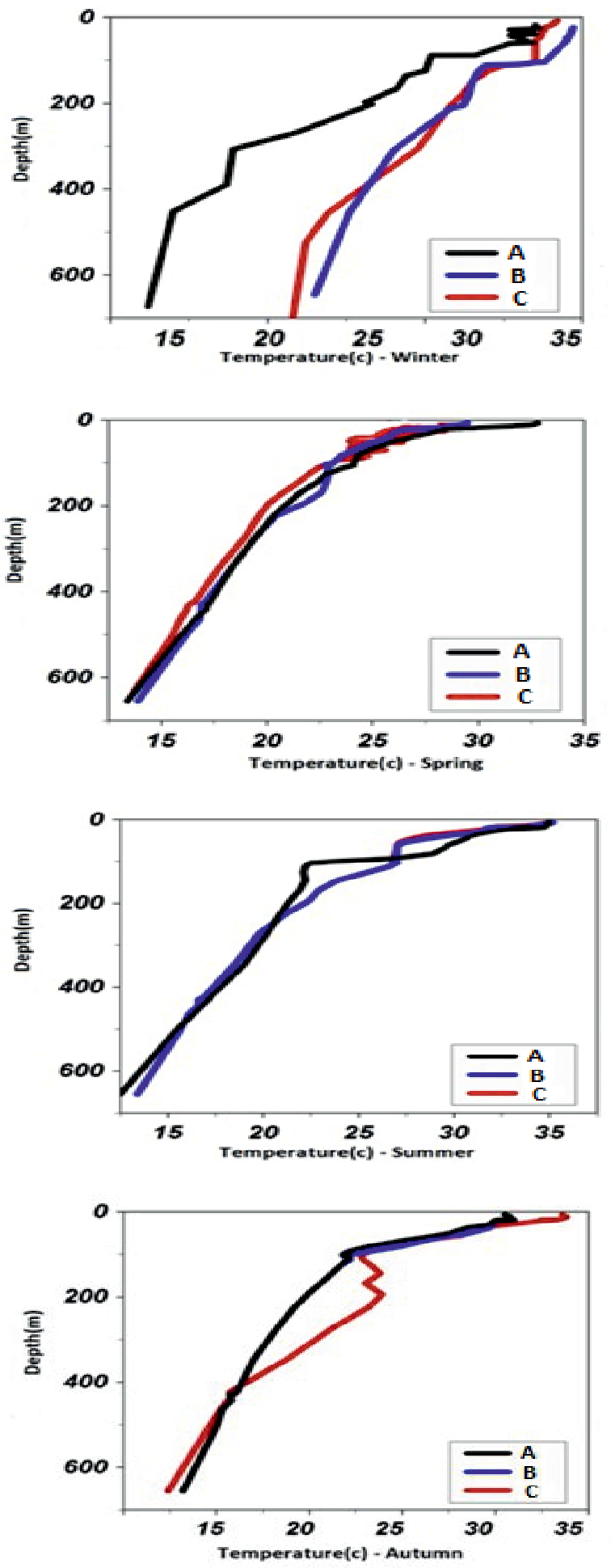
Seasonal vertical profiles of temperature at three different locations A, B and C have been analyzed in offshore and inshore waters over a depth of 600 meters in the North of Oman Sea.
At the start of the cold season, the surface temperature decreases steadily and temperature stratification is developed with a thermocline setting at around 80 to 100 meters. During this period, temperatures ranged between 20 and 25ºC at the surface. The modeled surface temperature at the start of the warm seasons continuously increased and reached the highest values in the middle of August (30 to 33oC) and then decreased gradually in the middle of November 25-30oC (Fig. 7). A strong stratification exists in winter; however, the vertical changes in the physical parameters of water are negligible. With the beginning of spring and the rising water temperature, the water column is decomposed and a thermocline layer is formed. The thickness of this layer grows in late spring (50 to 70 m). The sea surface temperature (SST) increases and becomes greater than 24oC, which might be the ideal condition for the blooming.
Table 2.
List of parameters used in the biogeochemical model [37].
Table 3.
Long-term mean and standard deviation of model and satellite chlorophyll concentration in Areas A, B and C.
| Area | A | B | C | ||||
|---|---|---|---|---|---|---|---|
| Mean | Standard deviation | Mean | ±SD (N = 162) | Mean | ±SD (N = 162) | Mean | ±SD (N = 162) |
| Model | 1.47 | 0.752 | 1.22 | 0.814 | 1.83 | 1.26 | |
| SeaWifs | 1.65 | 0.767 | 1.52 | 0.844 | 2.04 | 1.22 | |
Fig. 6.
Temperature cross-sections along 25.6-26.6°N during winter, spring, summer and autumn respectively.
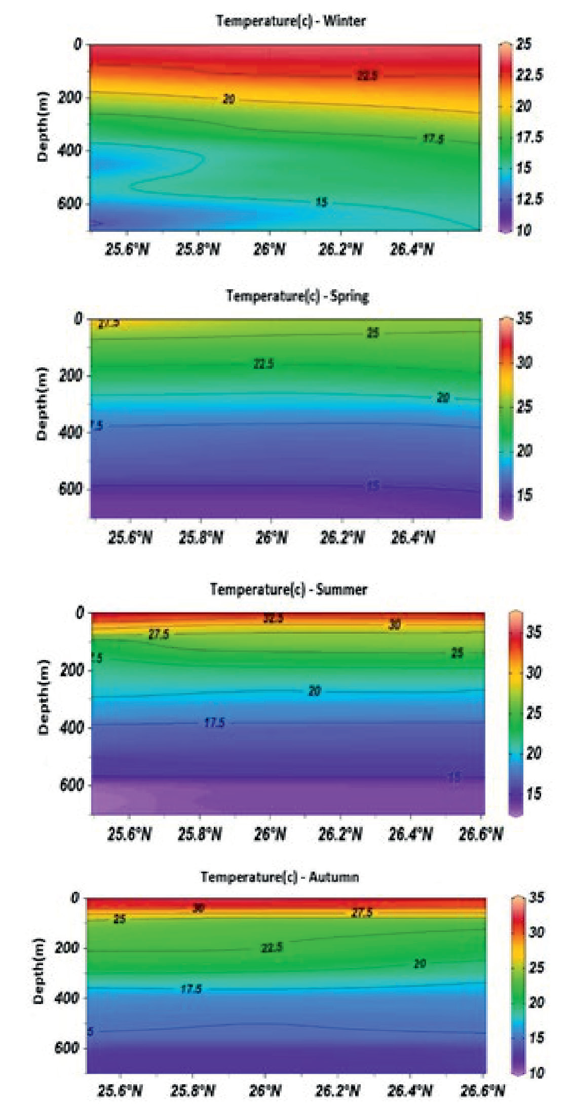
Fig. 7.
Seasonal vertical profiles of temperature at three different locations during winter, spring, summer and autumn respectively (A, B and C in Fig. 2) from the North of Oman Sea.
Velocity Profiles and Seasonal Variations
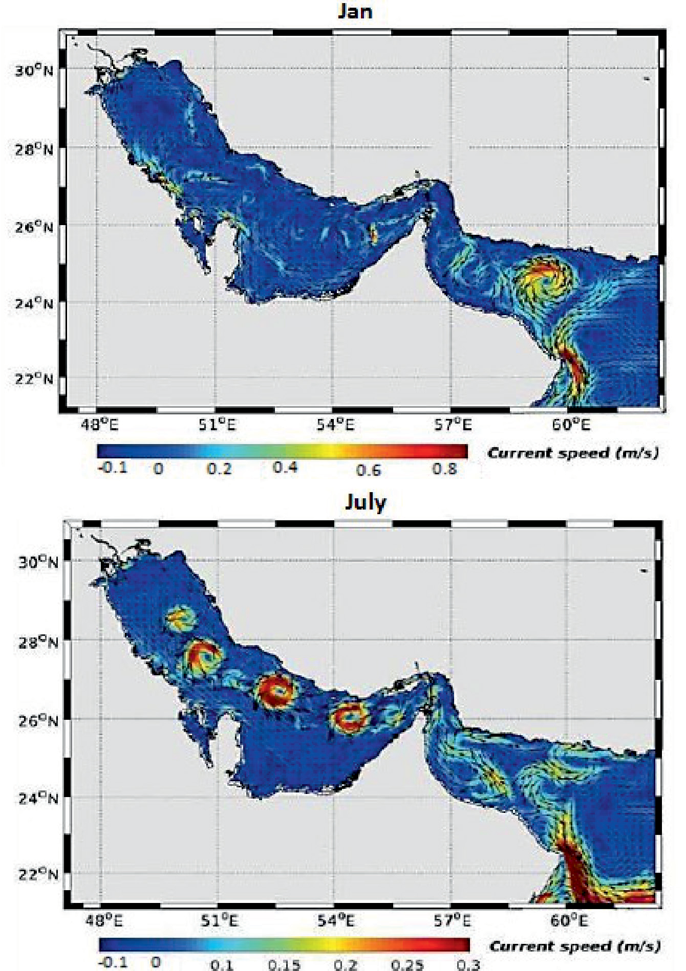
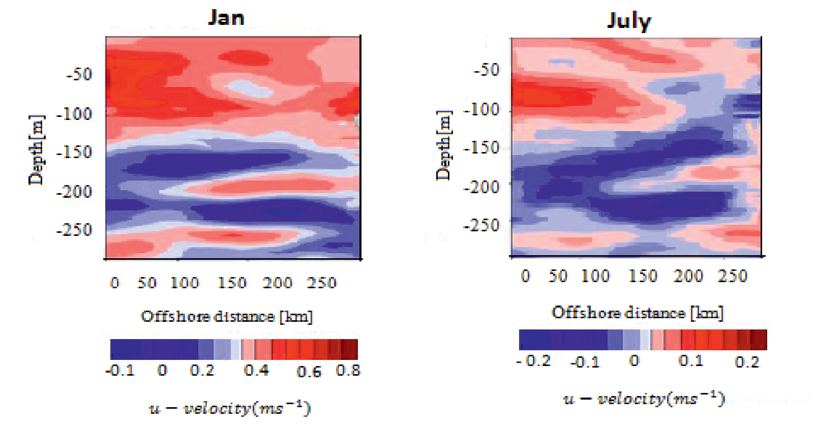
In January, two strong currents are evident. A very strong, anticyclone current can be seen in the middle of the Oman Sea during this month of the year. The maximum speed of this month’s currents is 0.8 m/s. Oman’s anticyclone current is strong and large in January and penetrates to a depth of 300 meters. As the depth increases, the current speed decreases and reaches about 0.5 m/s at a depth of 300 meters. In July, the current speed decreases drastically and reaches about 0.1 m/s (Fig. 8). Figs 9 show mean monthly of velocity field and cross-section of current speed along DE path for January and July respectively, to represent locations and depths of influence of major eddies along DE path and to investigate their effects on other variables. The modeled velocities reproduce fairly well observed data with average skill of 0.6 to 0.8 m/s for u-velocity. The lowest is found 200 m depth where the speed is 0.01 m/s for the simulated u-velocity.
Phytoplankton and Zooplankton Dynamics
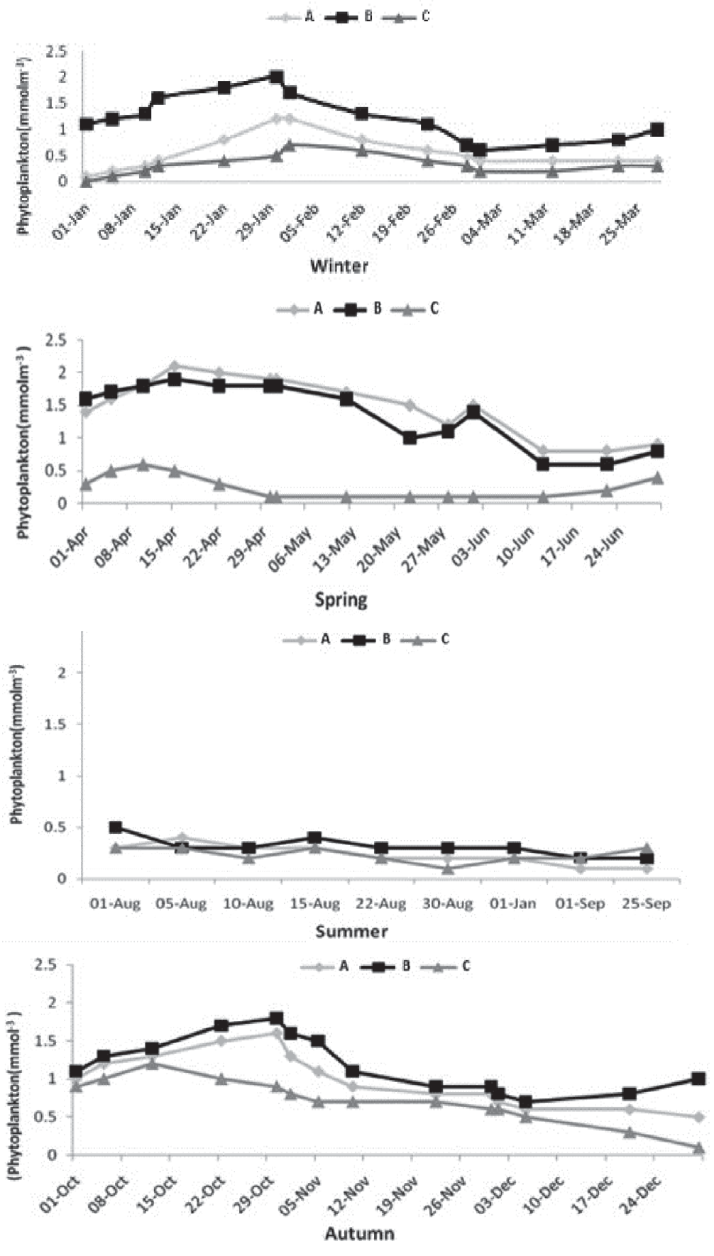
A vertical cross section shows the concentration of phytoplankton during winter and summer on the North Coast. Vertical distribution cross-section plots showed higher phytoplankton concentrations during winter and they were evenly distributed along the water column compared to summer where an apparent stratification is proposed for their vertical variations. Both advection and horizontal diffusion are important in determining the location of the maxima of phytoplankton and zooplankton and the productivity of the system. Phytoplankton concentrations in winter (0.6 to 1 mmolm-3) are higher than summer (0.1 to 0.4 mmolm-3) in surface water (Fig. 10). Upwelled water flows northward and affects the oceanic stratifications of the Gulf of Oman through gyres and eddy systems that sweep open ocean water into the Oman Sea. Upwelling systems with high velocity prevent large amounts of phytoplankton mass. It takes time for phytoplankton communities to adjust to the new conditions imposed by nutrients. In this section, we describe the main seasonal patterns in phytoplankton biomass in the three selected regions, as shown in Fig. 11. The model-derived patterns in phytoplankton biomass have important regional differences in terms of seasonal variability. To illustrate this, we estimated the monthly climatology of phytoplankton concentrations from the surface to 250 m deep within regions A, B and C (see Fig. 2). Phytoplankton concentration is at its highest during January and April in regions A and B and February and April in region C, and it is at its lowest during August in all three regions. The Southwest monsoon affects the region from June through September, although temporal shifts of monsoonal periods were noticed. Monsoonal winds contribute to the enrichment of the euphotic layer of the ocean with nutrients. Regionally, we dealt with seasonal winds as well as seasonal variations of the wind speed and the effects of mesoscale eddies on the dynamics of nutrients and hence, phytoplankton populations. The Gulf of Oman and the Strait of Hormuz were occupied by highly abundant, strongly diatom-dominated phytoplankton compilation.
Fig. 10.
Vertical phytoplankton distribution in the DE cross-section in January and July, respectively.
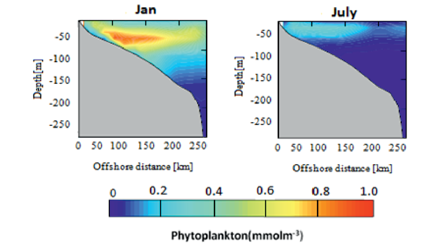
Fig. 11.
Monthly abundance of phytoplankton in three different locations (A, B and C shown in Fig. 2) from the North of Oman Sea.
Results revealed that the abundance and composition of winter phytoplankton was related to water circulation patterns in the Persian Gulf and the Gulf of Oman.
A multiple peak structure in the dynamics of zooplankton abundance is synchronized with monthly changes of phytoplankton organisms. The adaptation of zooplankton populations to availability of food to the number of predators is another issue that needs attention. Fig. 12 shows the time evolution of the inshore Areas A and B and offshore Area C (see Fig. 2). Zooplankton biomass along the North Coast of the Oman sea. In the inshore area, along the north coast, in Areas A, B and C, the seasonal cycles of zooplankton biomass differ. Within Areas A and B, maximum is reached in August and in Area C it is reached in September. Furthermore, in Areas A and B, the zooplankton biomass exhibits two distinct maxima, one in winter and another in early spring. A vertical cross section shows the concentration of zooplankton during and summer on the North Coast. Vertical distribution cross-section plots showed higher zooplankton concentrations during summer. Fig. 13 shows zooplankton concentrations in summer (0.8 to 1 mmolm-3) are higher than winter (0.1 to 0.3 mmolm-3) in surface water. The peak of zooplankton bloom can be seen from the surface to a depth of 40 meters and gradually decrease with depth in July. In January the density reaches almost zero in depth.
Model Validation and Comparison with Satellite Data
We configured an ocean-biogeochemical model for the ROMS model that predicts the concentrations of phytoplankton and zooplankton in a clear and precise manner.
Our model reproduces the main physical and biochemical patterns reasonably well, although an underestimation of the mean surface chlorophyll is evident in the northern shelf, especially at the bottom layer at a depth of about 600 meters. We studied the main model phytoplankton and zooplankton biomass patterns and surveyed the fundamental factors explicating biomass variability, following a similar approach were used by previous research [44].
We extracted the chlorophyll data over the study area from SeaWiFS archive with resolutions of 4 km to validate results of the model. After making some necessary corrections, monthly basin averaged surface chlorophyll over Sea of Oman derived from model was calculated and compared with satellite data for 6years period from 2006 to 2012 as shown in Fig. 14.
Fig. 13.
Vertical zooplankton distribution in the DE cross-section in July and January, respectively.
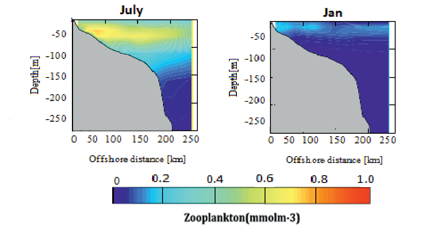
Fig. 12.
Annual cycle of zooplankton biomass integrated over 100 m in Areas A, B and C (2008) (see Fig. 2 for the definition of the different areas).
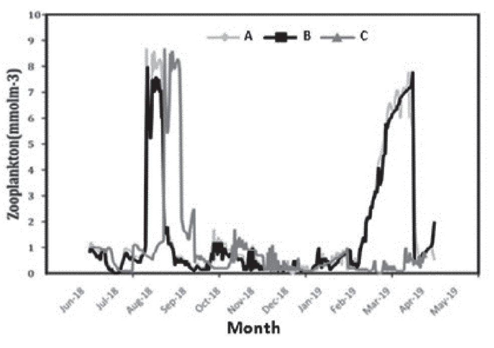
Fig. 14.
Monthly averaged surface chlorophyll time series derived from model (ROMS-NPZD, a) and (SeaWiFS, b) over sea of Oman for 2006-2012.
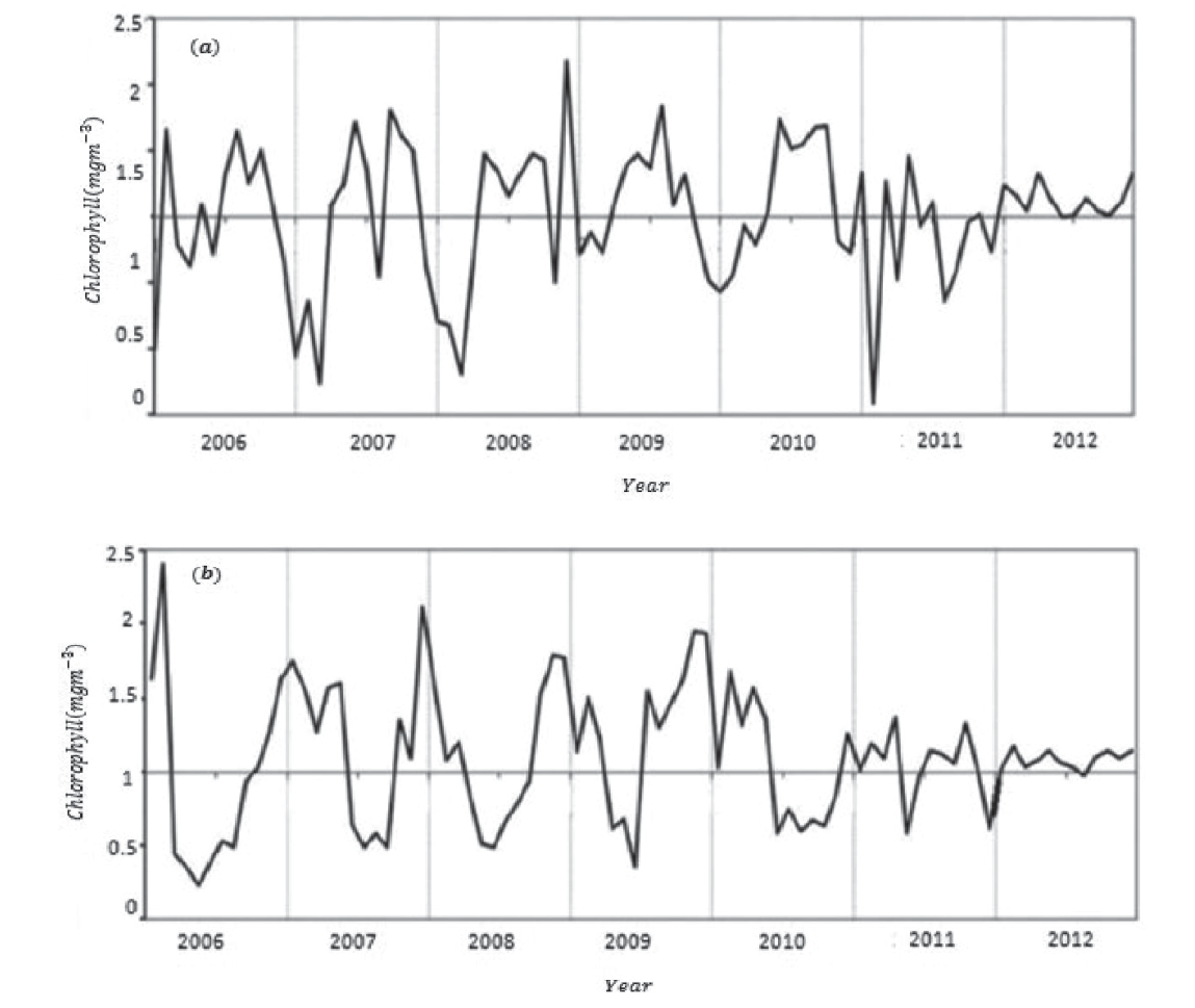
As can be concluded from Figs 14, monthly average surface chlorophyll obtained from satellite databases in Sea of Oman during these years has an average of about 0.2 mgClm−3 and maximum of about 2.5 mgClm−3. These values show a good consistency with the results obtained from the present model in the climatic run.
It’s worth noting that the default NPZD model which is included in the ROMS generally yields underestimated values of surface chlorophyll for the study area. So, we had to do many successive runs to yield the best configuration for the model parameters which was beyond the scope of this paper. It should be noted again that available previous research in Oman Sea did not use numerical studies to predict the distribution of phytoplankton and zooplanktons. Since eddies are one of the most important factors in the transfer nutrients from the Persian Gulf into the Oman Sea, further studies on this topic would be useful. A study conducted in the Atlantic Ocean has also shown similar findings. For instance, a three-dimensional ROMS model has been paired with the NPZD biological model to investigate the seasonal variations of phytoplankton and zooplankton in the Iberian (northeast Atlantic) region indicating phytoplankton and chlorophyll concentrations in spring and early summer and then, blooming happen again in late summer and early fall [45].
We found that zooplankton grazing plays an important role in controlling phytoplankton biomass seasonality. Zooplanktons are also very important in marine pelagic food webs because they are used as food for larval fish and as a good indicator for changes in water quality [46].
A comparison with in situ seasonal chlorophyll observations suggests that part of the model-satellite chlorophyll disagreement could be linked to chlorophyll overestimation by satellite sensors. We can see that the variation trend and chlorophyll concentration are almost the same. The inshore and offshore differences in chlorophyll concentrations are highly significant with a decrease from inshore to offshore. Strong seasonality in chlorophyll-a distribution with higher concentrations in winter and spring and lower in summer and autumn is well reproduced by the model which is confirmed by satellite observations as well.
The main differences between model and satellite time series are located in the coastal region, where model chlorophyll is much lower than SeaWiFS chlorophyll, perhaps due to the errors in the representation of the inter-annual variability of nutrient information. By comparing the modeled time series with satellite data, it can be concluded that satellite sensors might be overestimating surface chlorophyll. The satellite observations (SeaWiFS at 24°N, 58°E from Asia-Pacific Data Research Center) from 1997 to 2013 suggested that chlorophyll-a concentration in the Gulf of Oman increased in August 2000, September 2004 and August 2008 [47]. The results showed that a significant correlation exists between inshore and offshore chlorophyll-a distribution throughout the year.
Table 4.
Root mean squared error and correlation coefficient results.
| Area | RMSE | r |
|---|---|---|
| A | 0.223 | 0.985 |
| B | 0.371 | 0.968 |
| C | 0.490 | 0.981 |
The temperature regime of the coastal waters in the north of Oman clearly conforms to an annual cycle with low temperatures detected in the winter and the highest sea surface temperatures observed in the summer. Oman Seawater follows a form of temperature inversion layers. The intrusive thermohaline structure in the Oman Sea is influenced by two processes called double diffusion and salt fingering [48]. Results show a strong relationship between sea surface temperature, nutrient input in the surface layers and the corresponding enrichment of phytoplankton in the Oman Sea upwelling. The thermocline under the influence of coastal upwelling, or in deep water, injections of nutrients are generated by the coastal winds and mesoscale cyclonic eddies. At a temperature of 30 degrees Celsius, the growth of plankton is limited which indicates that the temperature is a limiting factor in summer. However, in autumn, as the weather becomes colder, they become abundant again. Cyclonic and anti-cyclonic eddies, which indicate an upwelling in the Sea of Oman and the Strait of Hormuz; cause the transfer of chlorophyll from the southern regions of the Sea of Oman to the northern areas, and finally the Strait of Hormuz and into the Persian Gulf [49].
In winter, results show decreasing depths of thermocline and neutrocline layers and also strong layering affect convections in these waters. In fact, under these conditions, cold eddies (usually cyclonic mesoscale eddies) are able to transfer nutrients to the optical layer of the surface and cause phytoplankton to bloom. During the summer monsoon, offshore upwelling and environmental forcing can replace the effects of eddies [50]. Also, the vertical changes of chlorophyll a and its seasonal changes in the northern half of the Oman Sea show that the highest distribution and density is in the surface layers and its concentration decreases as the depth increases. It seems that the temperature and the amount of decrease in light radiation have a direct effect on reducing the amount of chlorophyll a. Higher values of chlorophyll a concentration was observed in winter along with thermocline vertical movement under the influence of local wind-driven upwelling. In this case, injection of nutrients occurs through mixing across the thermocline. In the Oman Gulf, thermoclines are always formed. Seasonal changes only modify the thickness or width of thermoclines. Low chlorophyll a values were observed during summer despite a high presence of nutrients. This might be a result of low light due to lack of stratification and hence, a deep mixed layer [51].
Surface currents have great importance in marine studies. These currents can be an important factor in the transfer of density, nutrients or pollutants into the ocean environment. The water area of the Persian Gulf and the Sea of Oman is one of the most important waterways in the world. The general flow in the ocean currents in the Gulf of Oman is in the anti-cyclonic direction, that is, along the northern coast of Oman, the predominant coastal current moves southeastward from the Gulf of Oman. Indeed, the cyclonic and anti-cyclonic eddies in the Sea of Oman have a deep reaching dynamic signature. Note also that, in June 2008, a small anticyclone appeared near 58-59°E, between the large cyclone near 57°E and the large anticyclone again near 60°E. The strongest currents of the Oman Sea are forming in autumn and winter (in January and March). Currents are cyclonic in winter and marginal strong in autumn. The highest value of velocity in the Oman Sea is 0.8 m/s and the lowest value is 0.1 m/s.
Oman’s anticyclone eddies are strong and large in January and penetrates to a depth of 300 meters, another cyclone eddy can be seen which is smaller and flows at a slower speed. In the following months, this anti-cyclone eddies weakens and in March it has given itself to other strong currents that are associated with the general circulation of Oman. In the surface layer of the Oman Sea up to a depth of 500 meters, a mesoscale cycle is formed, whose circulation is cyclonic. The formation of cyclonic eddies on the surface is consistent with the observations of Rapmi, which is a proof of the accuracy of the model results. In the western part of the Oman Sea and on the left side of this main cycle, two small anticyclones are formed in the continental plateau region. The model captures seasonal variability of anticyclonic circulation in the Oman sea shows good agreement with results and observation reported [52]. In winter, the temperature of the water column is relatively homogeneous, which indicates the presence of mixing in the water column. The mixing of the water column from January to April is one of the growth factors of phytoplankton, of course, with increasing depth, decrease temperature and the increase turbidity which prevents the penetration of sufficient light in the water column, has a negative effect on the growth of phytoplankton. As the weather warms from late June, the amount of phytoplankton decreases because the temperature exceeds the tolerance threshold of phytoplankton. The vertical profile of the distribution of zooplanktons also shows that the population of zooplanktons increases with a short delay after phytoplankton, and as the abundance of phytoplankton, the amount of zooplanktons also decreases.
The blooming period of the planktonic population throughout the year has been found to occur in the spring season. The model is also able to reproduce blooms on the northeast coast of Oman during the North East Monsoon through convective mixing. The offshore and inter monsoon oligotrophic conditions are also captured by the model as well as the offshore deep chlorophyll maximum. The model results are in agreement with (the scarce) in situ and satellite data in terms of reproducing temporal and spatial variability in nutrients, phytoplankton and zooplankton concentrations at least qualitatively.
It seems that one of the most important and effective factors in increasing the number of plankton is the influence of southeastern currents on the Oman Sea in the summer monsoon [53]. Phytoplankton bloom slightly earlier than zooplankton; therefore, in early spring, due to the increase in phytoplankton and the provision of sufficient food for zooplankton, their amount increases, as compared to summer concentrations.
Conclusions
The results show that the way chlorophyll changes compared to modeled simulations is similar to those of satellite color images and the use of this numerical model to investigate seasonal variability on the changes of phytoplankton and zooplankton is appropriate. However, changes in the movement of plankton are due to the changes in the location of eddies, and because the movement of eddies is not a predictable phenomenon, sometimes there are discrepancies between the model output and satellite images. Also, the model’s limitations in stratification simulation and the amount of radiant light penetration can be the reason for the differences observed. Because field measurements of ecological parameters are time-consuming and expensive; nowadays the use of numerical models in predicting many hydro physical and biological parameters has become common. Modeling of ecological processes, like the ones carried out here, is of particular importance because physical factors and biogeochemical processes (as can be tested in different scenarios of surface biological activities) strongly influence plankton populations and marine production. In addition, ecological processes are very complex and have multiple interactions with each other. Modelling these processes requires more environmental data to be collected. The results of the present simultaneous study in modeling physical and biogeochemical processes can be used reliably to predict the dynamics of plankton populations in aquatic ecosystems.

