Introduction

The epoch of the Industrial Revolution catalyzed a massive leap in global industries and economies, unfortunately, along with an amplification of air pollutants from various industrial sources. The expansion and severity of worldwide pollution escalated, drawing increased focus [1-4]. An increase in air pollutant levels, coupled with the deteriorating state of the global environment, significantly impacts human health and overall quality of life. This underscores the urgent imperative to reduce pollutant concentrations and improve air quality [5-8]. Although numerous environmental protection policies have been introduced, alongside growing global awareness of atmospheric pollution reduction, excessive atmospheric pollutant concentrations persist, and environmental degradation remains a critical issue [9-10].

Air quality is principally impacted by pollutants like carbon monoxide (CO), carbon dioxide (CO₂), ozone (O₃), nitrogen dioxide (NO₂), sulfur dioxide (SO₂), and particulate matter (PM_2.5, PM₁₀). Among these, ozone plays a crucial role in the human health and ecological environment. Ozone is beneficial in small amounts, with a safe concentration at 0.2 mg/m³ [11], while a concentration above 100 μg/m3 is considered unsafe. The increase in ozone concentrations over the years can be attributed to industrial plant emissions and increased solar intensity [12, 13]. Elevated ozone concentrations can severely harm human health, particularly the respiratory system, and negatively impact the ecological environment, causing a decrease in crop yields and damaging agriculture and forestry [13].

The importance of ozone pollution prediction spans several areas: – Public Health: Ozone pollution, a detrimental

air pollutant, can harm human health, causing

respiratory problems, aggravating asthma and other

respiratory diseases, and increasing the risk of

cardiovascular issues. Accurate ozone prediction

enables timely warnings and necessary measures to

protect public health. – Environmental Impact: Ozone pollution affects not

just human health but the environment as well. It can

harm vegetation, reducing crop yields and disrupting

ecosystems. Predicting ozone levels allows for

proactive measures to mitigate these environmental

impacts. – Policy and Regulations: Ozone pollution prediction

aids in shaping policies and regulations aimed at

lowering pollution levels. It helps policymakers

identify sources of pollution and develop targeted

interventions. – Urban Planning and Infrastructure: Ozone prediction

informs decisions regarding urban planning and

infrastructure development. By understanding the

spatial and temporal patterns of ozone pollution,

city planners can minimize exposure to high ozone

levels. – Economic Implications: Ozone pollution can have

significant economic consequences, impacting

agricultural productivity and incurring health-related

costs. Accurate prediction of ozone pollution enables

better resource allocation and planning.

It is essential to protect the ecological environment while developing material civilization [14] as the sustainable coexistence of both ensures long-term prosperity for present and future generations. As awareness of environmental protection improves and concerns about air pollution status grow, establishing a scientific and effective atmospheric pollutants control mechanism becomes critical [15-16]. Air pollution prediction can effectively prevent serious pollution events, reduce the damage from heavily polluted weather, and minimize economic losses caused by severe air pollution [17-18].

Research has focused on ozone (O₃) forecasting [19]. Efforts have been made to enhance the accuracy of O₃ forecasting using classic methods such as regression analysis, time series analysis, autoregressive moving average models, and gray models [20, 21]. Despite their advantages, these methods often fail to capture nonlinear patterns prevalent in ozone data [22-24]. The advent of artificial intelligence (AI) technology has introduced intelligent methods for air quality and ozone forecasting [25]. Techniques such as expert systems, machine learning, and fuzzy reasoning have been utilized in this domain [26-30]. Among them, artificial neural networks (ANNs), capable of handling nonlinear factors, are often chosen for ozone forecasting [31]. Artificial Neural Networks (ANNs) mirror the human brain’s structure, comprised of several layers of interconnected neurons, each governed by activation functions. This design permits ANNs to navigate intricate data, notably nonlinear data, that traditional ozone forecasting techniques struggle to handle [32-35].

Back-propagation algorithm (BP), the dominant method among ANN models, grapples with sluggish convergence and protracted iteration cycles [36], When discussing the challenges of back-propagation algorithms in Artificial Neural Network (ANN) models, it’s important to note that ‘convergence speed’ refers to how quickly the algorithm reaches a stable and accurate solution during training. This impacts the efficiency of the learning process. Additionally, ‘iteration cycles’ indicate the number of times the algorithm updates its weights and biases by iteratively adjusting them during training. Efficiently managing these aspects is crucial for optimizing the training process in ANNs. Various refinements have been proposed to counter these limitations. For instance, Huang et al. employed Particle Swarm Optimization (PSO) to enhance the BP algorithm, boosting the convergence speed in air quality forecasting [37]. Likewise, Yang et al. constructed a BP-ANN model for PM2.5 forecasting, yielding satisfactory outcomes [38]. Qiao et al. employed a refined ant colony algorithm in conjunction with BPNN to predict peak load in Chengdu, showcasing a marked improvement in prediction accuracy compared to conventional regression models [39]. Ya et al. underscored the prowess of Convolutional Neural Networks (CNNs) in extracting nonlinear data features, emphasizing their advanced feature extraction capabilities [40], Convolutional Neural Networks (CNNs) are a class of deep learning models designed for processing grid-like data such as images. They excel at feature extraction through the use of specialized layers called ‘convolutions.’ These convolutions systematically scan the input data, identifying patterns, edges, textures, and more. This hierarchical feature extraction allows CNNs to automatically learn and represent complex features, making them highly effective for image analysis, object recognition, and other tasks. Their ability to capture spatial relationships and hierarchies in data has made CNNs a go-to choice for computer vision applications. Deep learning approaches, such as Recurrent Neural Networks (RNNs) and their variants like Long Short-Term Memory (LSTM) and Gated Recurrent Unit (GRU), have attracted interest for their performance in time series prediction tasks, particularly in deciphering underlying patterns in larger, more intricate datasets [41-43]. While RNNs have traditionally been employed, they’re hampered by the vanishing gradient problem, which LSTM effectively resolves [44]. LSTM employs gated neural units output gates, input gates and forgetting gates, to retain contextual data and extract long-term features from time series data [45].

Numerous studies have harnessed LSTM for ozone forecasting, demonstrating its efficacy. For instance, Zhang et al. developed an ozone prediction methodology based on LSTM, delivering encouraging forecasting results [46]. Pak et al. presented a blend of CNN and LSTM for short-term ozone forecasting, using CNN to draw out high-level features and enhance accuracy when the LSTM input sequence is long [47]. This synergy of CNN and LSTM has been shown to be a superior model for predicting air quality time series data [48, 49]. The amalgamation of AI methods, particularly ANNs and deep learning models like LSTM, has progressed the ozone forecasting field. These models excel at deciphering the nonlinear characteristics of ozone data, enhancing prediction accuracy against traditional linear analysis methods. Further investigation into hybrid models, merging techniques such as CNN and LSTM, might yield improved results in forecasting air quality and ozone levels. The ongoing advancement and honing of AI-based techniques will contribute to more precise and reliable ozone forecasting, aiding in the control and reduction of air pollution.

To overcome the restrictions of traditional artificial intelligence models, series decomposition methods are utilized to process time series signals. Signal processing methods play a vital role in combined models and directly impact the model’s predictive performance. Standard sequence preprocessing techniques include Wavelet Decomposition (WD) [50] and Empirical Mode Decomposition (EMD) [51]. The EMD decomposition algorithm doesn’t rely on any basis function and differs significantly from wavelet decomposition. It’s particularly efficient at handling non-stationary and nonlinear complex signals. Li et al. [52] put forward the AQI forecasting algorithm using Variational Mode Decomposition (VMD) and improved the VMD results by employing bald eagle search to propose a BVMD refined model for better outcomes. The research conducted in Xi’an, Beijing, and Shanghai shows that the proposed method is superior to other decomposition techniques.

Consequently, VMD dynamically dissects the relevant components associated with each center frequency within the frequency spectrum, demonstrating superior precision in decomposition. The VMD method’s ability to decompose data has proven particularly beneficial in feature selection for predictive models and has seen successful applications in forecasting trends in asset prices within financial and energy markets [53]. Therefore, this study adopts the VMD decomposition approach as the main tool for decomposition in our modeling process.

In this paper, we use CNN-LSTM to directly process deformation monitoring time series data in the time domain and extract the data dependence information therein. Combined with VMD, we propose a deformation prediction model based on VMD-CNN-LSTM. Initially, VMD decomposes the deformation monitoring data sequence into a set of relatively stable intrinsic modal components with different frequency scale characteristics, reducing the influence of nonlinearity and non-stationarity, and easing prediction; the optimal number of modal components in VMD is determined by calculating the permutation entropy of the decomposition margin; then CNN-LSTM is directly employed to predict each modal component, and mine the multi-scale features in the original data according to the characteristics of different modal components; finally, the predicted values of each component are overlaid to obtain the final result.

The primary contributions of this paper are:

• Complexity and environmental variation cause the Ozone (O₃) data series to have a high degree of variation. The VMD-CNN-LSTM model is used to analyze complex time series data of Ozone (O₃) by decomposing it into multiple sub-signal components in the frequency domain using the Variational Mode Decomposition (VMD) technique. The VMD decomposition results in the original sequence, various VMD components, and residual items. The residual series is further decomposed using the Ensemble Empirical Mode Decomposition (EEMD) technique and combined with the LSTM model for predictive analysis.

In a study comparing different machine learning models using Ozone data from four Chinese provinces, the proposed VMD-CNN-LSTM model outperformed other models. The performance was evaluated using various indicators such as Mean Absolute Error (MAE), Mean Squared Error (MSE), and Root Mean Squared Error (RMSE), indicating the superior predictive capability of the VMD-CNN-LSTM model for Ozone prediction in this particular context.

The paper is structured as follows: Section 2 provides a brief introduction to the hybrid model construction. Section 3 presents results and analysis for Nanjing city. Section 4 provides discussion. The final section draws conclusions.

Materials and Methods

Before we delve into the construction of the VMD-CNN-LSTM hybrid model for predicting changes in ozone (O₃) levels, it’s crucial to briefly describe the components of this combined model: Variational Mode Decomposition (VMD) technology and the CNN combined with LSTM neural network.

Proposed VMD-CNN-LSTM Model

Ozone behavior is characterized by its non-stationary nature, nonlinearity, and other intricate properties. Predicting ozone levels accurately using a single technique proves to be a complex task. Nonetheless, the technique known as Variational Mode Decomposition (VMD) has shown promise in effectively breaking down complicated ozone signals into numerous simplified modal components. By applying prevalent prediction methodologies to each modal component extracted via VMD decomposition, a notable improvement in prediction accuracy can be observed. Prior studies have mainly concentrated on the modeling of modal components estimated through VMD decomposition, often overlooking the intricate information within the residual terms post-decomposition.

To overcome this issue, a hybrid model of Convolutional Neural Networks (CNN) and Long Short-Term Memory (LSTM) neural networks can be deployed. Both CNN and LSTM networks are adept at capturing autocorrelation within time series data and possess the ability to remember long-term patterns. By merging the VMD decomposition method with the CNN-LSTM network structure, the prediction accuracy of ozone levels can be substantially amplified. This integrated approach enables separate modeling and prediction of each modal component, harnessing the uniformity extracted by VMD. Moreover, the complex information within the residual terms is processed by the CNN-LSTM network, effectively recognizing temporal dependencies and long-term patterns.

Fig. 1.

Hybrid Forecasting Model: VMD-CNN-LSTM for Improved Time Series Prediction.

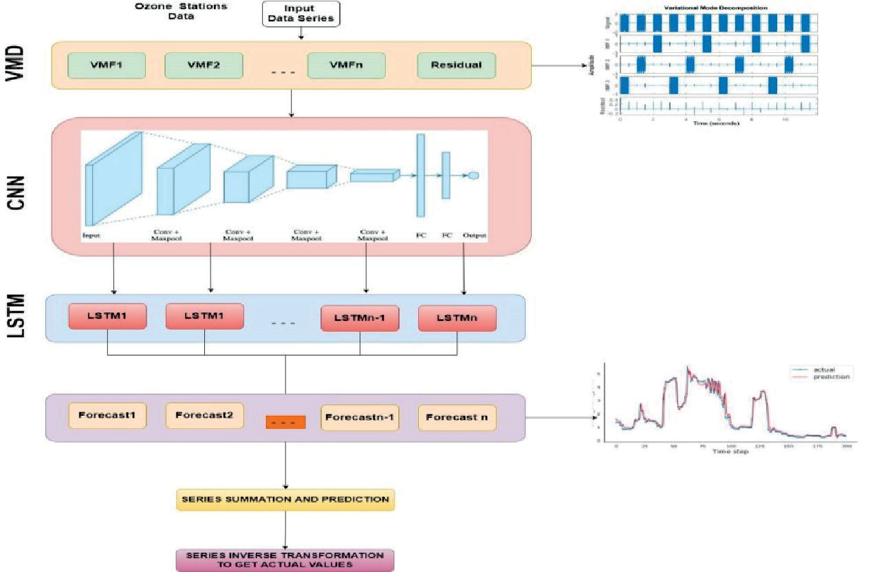
Here’s an outline of the comprehensive modeling steps of the proposed methodology:

Step 1: VMD Decomposition The initial ozone sequence is deconstructed using the VMD decomposition technique. This yields individual modal components, referred to as Variational Mode Functions (VMFs). Furthermore, the total VMF data is deducted from the original time series data, resulting in the residual term post-VMD decomposition.

Step 2: Normalization and Data Splitting The disassembled VMF components are normalized, and suitable training and testing samples are chosen. The normalized VMFs then serve as the input to the CNN-LSTM model. The CNN component of the model enhances the series prediction via convolutional operations, and the LSTM module is utilized to predict each Intrinsic Mode Function (IMF) subsequence within the VMFs individually. The predictions for each VMF component subsequence are derived.

Step 3: Residual Term Prediction The residual term obtained from VMD decomposition undergoes further prediction. Initially, CNN is employed to enhance the series prediction by applying convolutional operations to the residual term. Subsequently, LSTM is used to predict each subsequence within the residual term. The prediction outcomes of these subsequence predictions are combined to yield the final prediction result for the residual item.

Step 4: Aggregation of Prediction Results To obtain the final prediction result for the original sequence, the predictions derived from each VMD component and the residual item are aggregated. This involves summing up the predictions of each VMD component and the residual item obtained after VMD decomposition. By overlaying these predictions, the ultimate prediction result for the original sequence is obtained. By adhering to these modeling steps, the proposed methodology aims to achieve accurate ozone prediction by effectively deconstructing the original sequence, individually training each component using CNN-LSTM, and amalgamating the predictions to generate the final result.

Complete flow of the implementation is shown in Fig. 1.

Results

In this part, the areas selected for data collection and the results of the suggested approach’s execution will be discussed.

Series Decomposition and Forecasting Results

The Variational Mode Decomposition (VMD) technique is used to break down the original yield sequence into various VMF components and residual elements. Subsequently, the residual component and the series undergo a second round of decomposition using the Ensemble Empirical Mode Decomposition (EEMD). This decomposed data is then integrated with the Long Short-Term Memory (LSTM) model for predictive analysis. To evaluate the proposed method, we contrast it with the EEMD-LSTM model, which combines EEMD with LSTM technology.

To compare and analyze the effectiveness of the various combination models, we take into account the Mean Absolute Error (MAE), Mean Squared Error (MSE), Mean Absolute Percentage Error (MAPE), and R-squared (R²) values. Fig. 2 presents the average outcomes obtained from all the Nanjing stations and provides a comparative analysis of various models. The MAE values for the models show the lowest error for the VMD-CNN-LSTM model, affirming its exceptional prediction accuracy.

Similar patterns are observed for the MSE, MAPE, and R² values, with the VMD-CNN-LSTM model consistently outperforming the other models. In the VMD-CNN-LSTM model, the MAE and MSE values are reduced by 46% and 50% respectively, and the MAPE value is reduced by 4% compared to the EEMD-LSTM model. Furthermore, the R² value increased by 4%, indicating an excellent match between true and predicted values. The results highlight the exceptional performance of the proposed VMD-CNN-LSTM model in accurately forecasting ozone data, surpassing other models, including EEMD-LSTM.

Fig 2.

Comparison of different algorithms with proposed model of Nanjing a) MAE, b) MSE, c) MAPE, d) R^2.

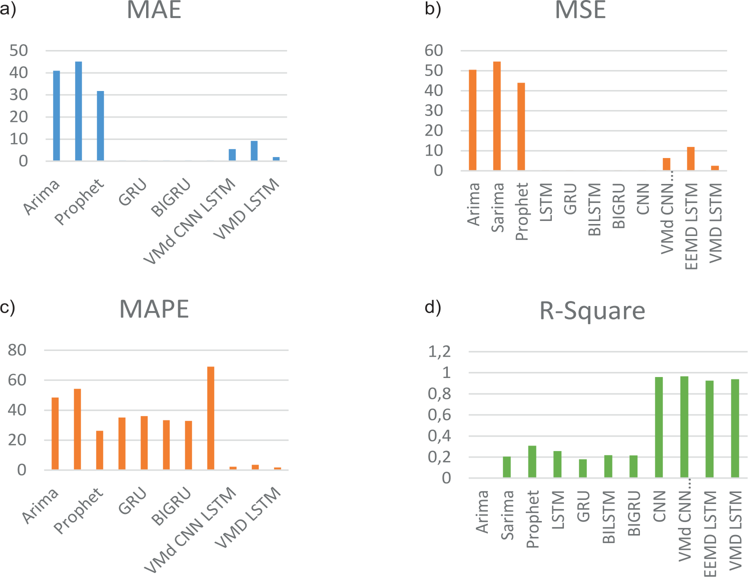
Fig. 3.

Comparing Actual and Predicted Values for All Algorithms a) ARIMA, b) SARIMA, c) Prophet, d) LSTM, e) GRU, f) BI-LSTM, g) BI-GRU, h) EEMD-LSTM, and i) VMD-CNN-LSTM.

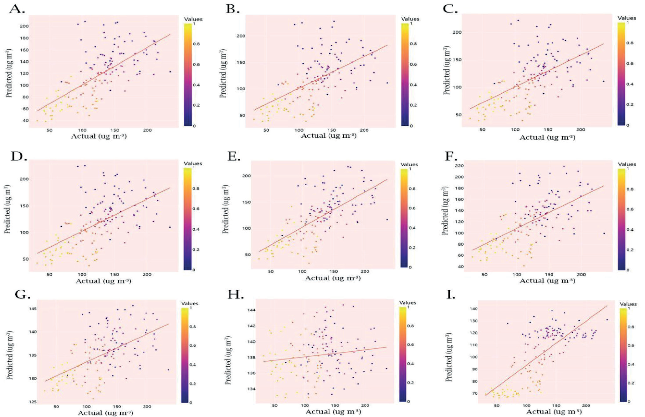
The value of R² is a reliability coefficient between zero and one hundred (or 0 and 1.0). A higher R² indicates a more reliable model. Due to the significance of both model stability and flexibility, optimizing R² is not the goal. To achieve optimal results in comparing the adjusted R² with the original R² value, it is desirable for the two numbers to be relatively close. Upon comparing the R² values of all prediction models, it is evident from Fig. 3 that the VMD-CNN-LSTM approach yielded the highest value (R² = 0.98).

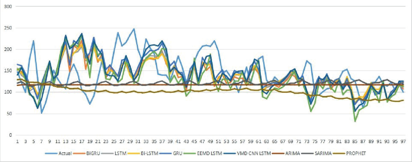
Fig. 4 offers a visual comparison of 150 days of observational data, underscoring the areas where our prediction model aligns with the actual values. Given the data’s non-linear and dynamic nature, our prediction model’s accuracy improves over time, increasingly aligning with the actual figures. The results further show that while LSTM models are adept at memorizing long-term patterns and generally provide accurate predictions, they fall short when it comes to complex Ozone data. Decomposing complex time-series data into subseries with varied frequencies via EEMD enhances prediction accuracy across all stations. When comparing performance across stations, LSTM appeared to underperform compared to GRU when inappropriate settings were used. The accuracy of the predictions was further improved by applying VMD to discern denoising patterns within the data for LSTM. The VMD-CNN-LSTM model excelled in predicting short-term Ozone levels, demonstrating its applicability in various other scenarios.

Fig. 4.

Visual comparison of 100 days prediction results of all the methods.

Discussion

This investigation delves into enhancing the accuracy of ozone predictions through the application of decomposition techniques. The complexity of ozone series can hinder the efficiency of direct prediction models. Several decomposition methods, such as Ensemble EMD (EEMD), Empirical Mode Decomposition (EMD), and Variational Mode Decomposition (VMD), have been tried, but their effectiveness is often limited due to modal aliasing and performance inefficiencies.

Variational Modal Decomposition (VMD) has proven to be a promising method for successful decomposition of ozone series, thereby mitigating issues present in previous techniques. After the initial decomposition, the Intrinsic Mode Function (IMF) components that remain complex can be further broken down, leading to a reduction in the complexity of the ozone series. Nevertheless, identifying which IMF components have high complexity is a daunting task.

Research conducted by Wang et al. [54] performed a straightforward decomposition of the IMF components, revealing that the primary component displayed the most complexity. In this research, VMD is used to measure the complexity of each IMF component and set quantitative criteria for choosing complex components. While VMD adeptly resolves modal aliasing and performance inefficiencies, it is crucial to properly predetermine the decomposition level and penalty factor for achieving optimal decomposition results.

Studies by Wu et al. [55] have shown that the use of series decomposition in comprehensive frameworks can greatly improve model predictive performance. For instance, an EEMD-LSTM model applied to pollution data from Anyang demonstrated marked improvements in terms of MAE, RMSE, and MAPE over the LSTM model. Other models, like VMD-SE-LSTM and EEMD-LSTM, also exhibited good prediction performance, prediction stability, and early warning accuracy across various datasets. These observations are consistent with this research, which also found EEMD-LSTM superior to LSTM following series decomposition.

An EMD decomposition model proposed by Huang et al. [56, 57] was utilized to filter noise from air quality data, leading to the extraction of IMF components. Using an EMD-IPSO-LSTM air quality prediction model, each IMF component was then modeled, resulting in improved prediction accuracy and superior model fitting compared to LSTM and EMD-LSTM models. Our research proposes a similar strategy, using EEMD, which also yields improved results compared to LSTM and EEMD-LSTM.

Our study’s methodology effectively predicts ozone levels, albeit with some limitations that warrant attention. The available experimental data was inadequate due to constraints in the experimental setup, and further refinement is needed. Additionally, our study lacked data on meteorological factors near the monitoring stations, which could have significantly bolstered our model’s performance.

The newly proposed VMD-CNN-LSTM model in this research brings several advantages to the prediction of monthly ozone levels: – Enhanced Prediction Accuracy: By decomposing

historical data series with the VMD technique, the

VMD-CNN-LSTM model seeks to improve the

prediction accuracy of monthly ozone levels. – Management of Outliers and Redundant Sites: Ozone

prediction often suffers from outliers and redundant

data from multi-source pollutant concentration

monitoring. The VMD-CNN-LSTM model

minimizes these influences by decomposing the data

and training each component individually. – Dealing with Cross-Interference: Cross-interference

between different pollutants needs consideration

when predicting ozone levels based on multi-

source data. This model effectively manages this

interference by separately training each decomposed

component. – Long-Term Memory and Adaptive Learning: The

LSTM part of the model demonstrates strong

adaptive learning and memory capabilities. This

allows the model to learn effectively from long-term

data and accurately predict ozone levels. – Comparative Performance: A comparison with other

models such as EMD-LSTM, EMD-CNN-LSTM,

and VMD-LSTM was carried out. The VMD-

CNN-LSTM model outperformed these models

in prediction accuracy and had lower error rates,

proving its effectiveness in capturing extreme ozone

levels.

Conclusions

While soft computing-based prediction models strive to improve accuracy, many often neglect the critical step of data preprocessing. Raw data is often filled with noise and superfluous information, emphasizing the need for effective data preprocessing in prediction models. This study introduces a decomposition algorithm for preprocessing, designed to reduce data dimensionality and extract key features from raw input. Despite significant advancements in natural language processing and computer vision via decomposition algorithms and deep learning, air quality time-series forecasting has seen limited progress in this regard. The primary aim of this paper is to present a novel predictive model that harnesses the benefits of EEMD, VMD, and LSTM. Decomposition algorithms can help disentangle complex air quality data into meaningful components, aiding in the identification of long-term trends, seasonal variations, and irregular patterns. Meanwhile, deep learning techniques, like recurrent neural networks (RNNs) or long short-term memory (LSTM) networks, can capture intricate temporal dependencies in the data, enabling more accurate and timely predictions of air quality levels. This combination of approaches can significantly enhance our ability to forecast air quality, benefiting public health and environmental management. Our analysis of Ozone data from nine stations in Nanjing has led to the following conclusions:

The integration of VMD and EEMD decomposition into various frequency components notably improved ozone prediction accuracy when utilized as input for the LSTM model. – Based on historical data, LSTM’s hidden layer

neural units were selected automatically, facilitating

predictions of both short-term and long-term

trends. Hidden layer neural units in Long Short-

Term Memory (LSTM) networks are automatically

determined through training on historical data.

The network adjusts the number of units in these

layers during training to capture the relevant

patterns in the data, enabling it to predict both short-

term and long-term trends effectively. This dynamic

adjustment is a key feature of LSTMs, as it allows the

network to adapt to the complexity of the underlying

temporal dependencies in the dataset. – The hybrid VMD-CNN-LSTM model put forth in

this study outperforms other models, showing a

high degree of fit between real and predicted values.

This approach has proven effective in accurately

forecasting AQI (Air Quality Index) in practical

scenarios. – Predicting future ozone levels, affected by intricate

factors like humidity and weather conditions,

poses a challenge. Future research may benefit

from integrating the proposed model with these

multidimensional complex influencing factors to

improve overall forecasting effectiveness. – Future work could consider exploring optimal

ensemble models for the decomposed modes,

optimal ensemble model refers to a combination

of multiple prediction models, each trained on a

specific mode obtained through data decomposition.

These ensemble models are designed to leverage

the strengths of individual mode-specific models,

enhancing predictive accuracy and robustness by

effectively blending their forecasts. The goal is to

harness the collective predictive power of these

models to improve the overall quality of predictions,

particularly in scenarios involving multifaceted

and complex data patterns, rather than using a

simple addition approach. Moreover, developing an

intelligent forecasting system and smart decision-

making system for ozone monitoring could help in

devising appropriate management policies based on

forecasted outcomes. However, while the proposed

VMD-CNN-LSTM method holds potential in enhancing ozone prediction accuracy, several limitations must be acknowledged: – Data Availability: The method’s efficacy is closely tied to the availability of accurate and comprehensive ozone data. Insufficient or inconsistent data can limit the model’s performance and applicability. – Parameter Selection: Proper selection of parameters like the decomposition level, penalty factor, and network architecture is crucial in the VMD-CNN-LSTM method. Inappropriate parameter selection can lead to inferior results and may necessitate manual tuning. Robust optimization techniques can be used for automated parameter selection. These techniques play a critical role in fine-tuning model parameters to achieve optimal predictive performance. By automating this process, we ensure that our models adapt effectively to the data, resulting in more accurate and reliable predictions. – Interpretation Complexity: The multistage process of decomposition, prediction, and recombination in the VMD-CNN-LSTM method can complicate interpretation and understanding of inherent data patterns and relationships. Decomposition separates the data into distinct components, prediction models operate on these components individually, and recombination integrates their predictions. This complexity can make it challenging to directly interpret the final prediction in terms of the original data, as the influence of each component on the overall prediction may not be immediately transparent. Therefore, understanding the intricate relationships among these stages becomes crucial for meaningful interpretation. – Sensitivity to Outliers and Noise: Like any predictive model, the VMD-CNN-LSTM method could be sensitive to data outliers and noise, possibly affecting prediction accuracy and necessitating additional preprocessing or outlier detection techniques. – Generalization to Other Locations: The method’s performance may vary when applied to ozone data from different geographical locations or cities with distinct environmental conditions, potentially requiring custom adjustments for optimal performance. – Computational Complexity: The implementation of the VMD-CNN-LSTM method could be computationally intensive, particularly with larger datasets or lengthy time series, requiring adequate computational resources and efficient strategies for practical application. By streamlining the computational demands of the modeling process, we can achieve faster predictions and reduce resource requirements, making the approach more feasible for real-time or large-scale applications. This optimization enhances the model’s efficiency and usability, which is particularly valuable in operational settings, such as air quality management or environmental monitoring. – Limited Consideration of External Factors: The

VMD-CNN-LSTM method mainly focuses on

decomposing the ozone time series and capturing

its inherent features, often not considering external

factors like meteorological conditions, air pollution

sources, or human activities. Including such factors

may improve the model’s predictive capabilities.

Furthermore, the method suggested in this research paper can be expanded to encompass additional areas of energy prediction, such as forecasting crude oil prices and wind speeds. By refining this approach and broadening its applications, we can enhance predictions and decision-making processes in various sectors, thereby leading to improved management strategies and better resource utilization.