

Introduction
North China’s urban agglomeration has often experienced serious atmospheric pollution [1]. In particular, heating in winter, emissions brought by human activities, and static atmospheric environments have caused frequent haze pollution events [2, 3]. Over the past decade, China has implemented rigorous measures for atmospheric pollution control and shut down a great number of high-pollution industrial facilities, thus improving the atmospheric quality of North China’s urban agglomeration [4]. Tangshan City in Hebei Province is a typical case. It used to be a typical heavy industrial city with serious atmospheric pollution due to high-pollution industries such as iron and steel, electric power, cement, and mining [5]. The atmospheric pollution caused by the heavy metals therein has had an adverse impact on human health and ecological security [6-10]. The monitoring of atmospheric element deposition during the winter heating period of this city can typically reflect the atmospheric quality of North China’s urban agglomeration.
The traditional (instrumental) methods play a major role in the atmospheric pollution monitoring system of China. However, this system is costly and technically complex. It has a limited quantity of monitoring sites with uneven geographical distribution and often does not include heavy metals in monitoring programs. Compared with the traditional methods, the lichen biomonitoring technique has advantages, such as low cost, easier sampling, easier analyses of elements, non-dependence on power supply, and collecting information on diverse heavy metals integrated over a period of a few weeks to years with minimal effect of momentary changes in deposits [11-15]. The main disadvantage of this technique is that it presents an indirect indicator rather than a direct measure of atmospheric deposition [16]. However, each technique has advantages and disadvantages. Active biomonitoring using lichens has long been regarded as a complementary or even an alternative method to traditional methods [17, 18].
As an effective biomonitoring tool, lichens have been widely applied to the biomonitoring of atmospheric element deposition [18-23]. Lichens are a symbiont of fungi and algae/cyanobacteria. Without roots, protective cuticles, and stomata, lichens obtain nutrition mainly from atmospheric deposition [18, 24] and have a strong ability to intercept and retain atmospheric deposits. Therefore, lichen element concentrations often show a positive correlation with atmospheric deposition levels [25, 26]. Active lichen biomonitoring is often used in polluted areas without indigenous or expected lichens [19, 23, 27], including some areas of China [28, 29]. In detail, lichens in an unpolluted area are transplanted to a polluted area and exposed for a period of time. Then the level, source, and temporal and spatial patterns of atmospheric element deposition in the exposure areas are evaluated according to the variations in lichen element composition before and after exposure [30].
Fig. 1.
Ramalina sinensis, the background area, the exposure area, wind rose map and atmospheric suspended pollutant concentration: (a) Ramalina sinensis; (b) location of the background area and the exposure area; (c) exposure area and exposure sites; (d) wind rose map of Tangshan City; (e) monthly average concentration of SO2, PM10 and PM2.5 of Tangshan City and Weichang County during the experiment.
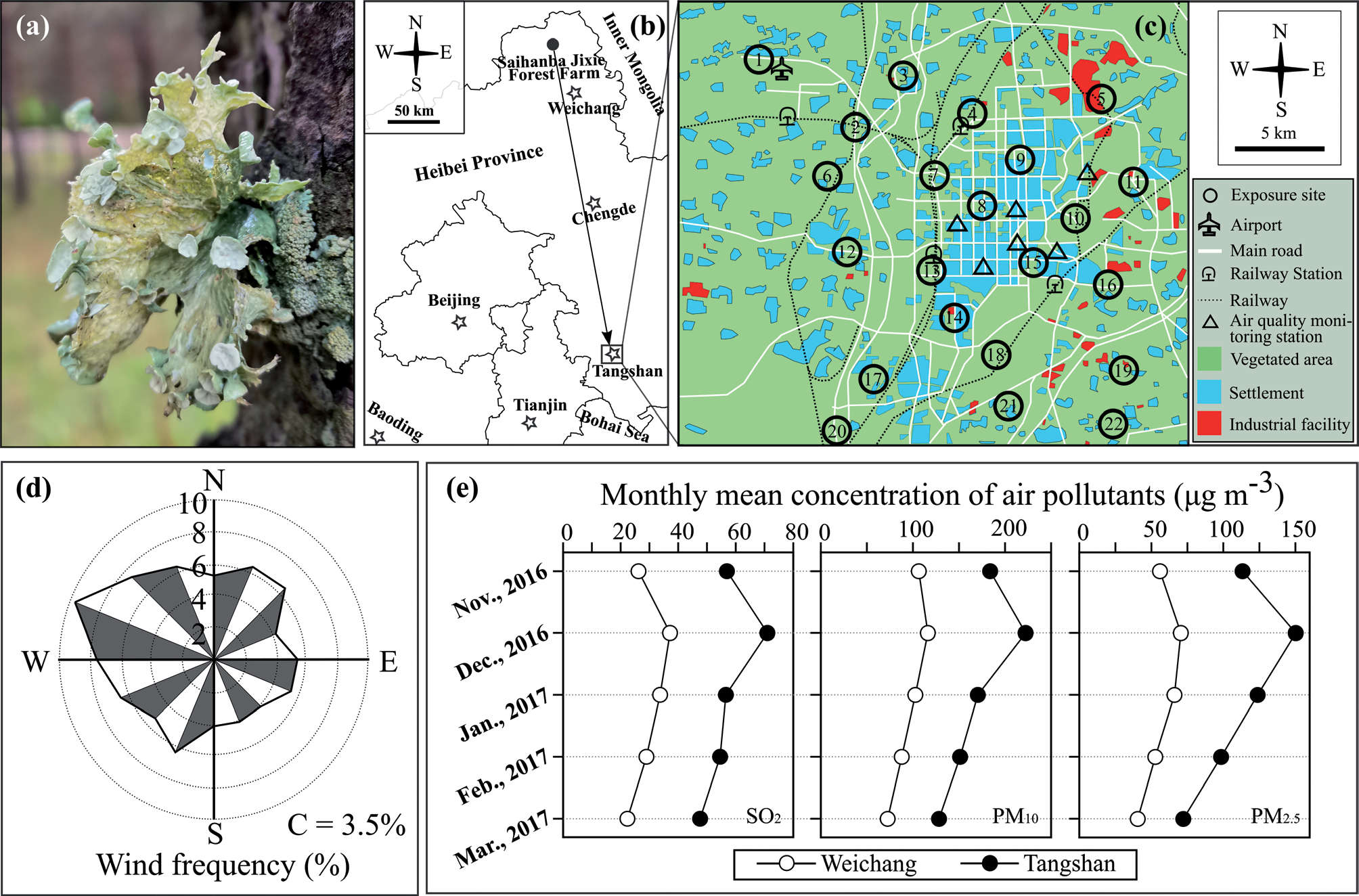
The suitability of Ramalina sinensis (RSI) as an active biomonitor in North China cities has not been tested. This lichen is widely spread in North China’s mountainous forests with a large biomass [31]. As a corticolous foliose lichen (Fig. 1a), RSI is attached to barks with a single bundle of rhizoids and can be easily collected. Its element concentration is not directly affected by soil or rocks, thereby meeting the purity criteria. It has a low baseline element concentration, and its exposure concentrations can reflect the chemical characteristics of atmospheric element deposition in the exposure area [32].
In this study, RSI collected from an unpolluted area was transplanted to 22 exposure sites in Tangshan (Fig. 1b & c) during the winter heating period, and then the concentration of 51 elements (Ag, Al, As, Be, Bi, Ca, Cd, Ce, Co, Cr, Cs, Cu, Dy, Er, Eu, Fe, Gd, Ge, Ho, K, La, Li, Lu, Mg, Mn, Mo, Nb, Nd, Ni, P, Pb, Pr, Rb, S, Sb, Sc, Se, Si, Sm, Sn, Sr, Tb, Th, Ti, Tl, Tm, U, V, Y, Yb, and Zn) in lichens was determined before and after exposure. This study was conducted to 1) explore the level and spatial distribution of atmospheric element deposition in the study area and analyze the source, and 2) verify the effectiveness of RSI as an active biomonitor in this area. This study is novel in that it is the first study using RSI as an active biomonitor in industrial cities in North China and testing the concentration of the most elements among the relevant studies.
Materials and Methods
Background Area and Sample Collection
Saihanba Forest Farm in Hebei Province is selected as the background area (117°15′11.93″E, 42°24′31.38″N; Fig. 1b). Featuring a typical cold temperate zone continental monsoon climate, this area has an annual average precipitation of 438 mm. Its altitude is 1,100- 1,940 m. It is located in the forest-steppe ecotone, with forest coverage of up to 82%. As a sparsely populated area, it is 50 km away from the downtown of Weichang County (Fig. 1b), the nearest population accumulation area. It has few industrial and agricultural activities and light traffic. Therefore, it is an ideal background area. During the exposure, the concentration data of atmospheric suspended pollutants (PM2.5, PM10, and SO2) in the background area was collected from the meteorological monitoring stations of Weichang County (Fig. 1e).
Lichens were collected 500 m around a sampling point (117°09′29″E, 42°26′07″N) with dense corticolous lichens on October 23, 2016. A large number of RSI were collected by hand at random from the bark of Larix gmelinii (Rupr.) Kuzen. and Betula platyphylla Suk at a height of 1-2 m from the ground. The samples were put into kraft bags, brought back to the laboratory, processed for air-drying at room temperature, and sealed in kraft bags at room temperature for further use.
Impurities were carefully removed from the lichen surface under a stereo microscope. Samples were rinsed 3-5 times, each for 5 sec with deionized water to reduce element concentrations in thalli and concentration variation between thalli [33]. Lichen thalli were divided into 71 composite samples, including 5 control samples and 66 exposure samples (22 exposure sites × 3 composite samples per site). Each composite sample consists of 10- 15 thalli of 2-4 cm in diameter to reduce the effect of concentration differences between thalli. Samples were packaged into nylon bags with a mesh size of 1 × 1 mm and a bag size of 10 × 15 cm.
Exposure Area and Lichen Exposure
Tangshan is selected as the exposure area. Located in the east of Hebei, North China (Fig. 1b), it has a dense population, a developed transportation network, and serious atmospheric pollution as a typical heavy industrial city. The iron and steel industry plays an important role in its industrial structure. It also integrates energy, chemical industry, building materials, and equipment manufacturing into a whole. It had a permanent population of 7.9 million and produced 91.2 million tons of crude steel in 2017, accounting for 11% of China’s steel production and 5.4% of the world’s steel production [6]. The atmospheric pollution was serious here [5, 34], with emissions of SO2 and NOx up to 159 × 103 and 204 × 103 tons in 2017 [5]. According to the Communiqué on the State of China’s Ecological Environment 2018, Tangshan City ranked in the bottom 4 of the 169 key cities under monitoring in 2018 in terms of atmospheric quality nationwide.
Twenty-two exposure sites (Fig. 1c) with a minimum distance of 3-10 km were selected to constitute a mesh square framework covering an area of 441 km2 (117°59′46″~118°14′32″E, 39°32′03″~39°43′29″N). The greatest efforts have been made to make these sites cover different environments, including factories, roadsides, residential areas, schools, parks, and airports. Most industrial facilities are distributed to the east of downtown.
The nylon bags containing RSI samples were hung to the trunks of Populus spp. at a height of 2.5 m at each exposure site (Fig. 1c) on November 14-15, 2016 so as to reduce the effect of hanging height and ground soil on lichen element concentrations and enhance the comparability between exposure sites [35]. Three duplicates (n = 3) were set at each exposure site, and each duplicate was one composite sample as above. After being exposed for 17 weeks, these samples were recovered on March 14-15, 2017. All the recovered samples were put into sealed paper bags and brought back to the laboratory, air-dried, and kept at room temperature until analysis.
According to the data collected from 6 meteorological monitoring stations (Fig. 1c), the concentration of atmospheric suspended pollutants (PM2.5, PM10, and SO2) in the exposure area was higher than that in the background area during the experiment (Fig. 1e). Northwest-west wind, northwest wind, and west wind are the prevailing winds in the exposure area (Fig. 1d).
Table 1.
Background and exposure concentrations of 51 elements in Ramalina sinensis.
[i] Note: Different capital letters indicate significant differences between the background and exposure concentrations (independentsamples T test, p≤0.05). In the column “Number of sites”, Ex>Bg indicates that the exposure concentration is significantly higher than the background concentration, and Ex≤Bg indicates that the exposure concentration is not higher than the background concentration.
Sample Preprocessing and Element Determination
Impurities were carefully removed from the surfaces of all recovered samples under a stereo microscope, and then these samples were dried in an oven at a constant temperature of 70℃ for 72 hours to a constant weight. The samples were ground in a ball grinder (Retsch MM400) with a tungsten carbide tank, filtered by a sieve with a mesh size of 2 mm, mineralized by microwaves in the mixture of HNO3-H2O2, and finally sealed for testing.
The concentration of 51 elements (Ag, Al, As, Be, Bi, Ca, Cd, Ce, Co, Cr, Cs, Cu, Dy, Er, Eu, Fe, Gd, Ge, Ho, K, La, Li, Lu, Mg, Mn, Mo, Nb, Nd, Ni, P, Pb, Pr, Rb, S, Sb, Sc, Se, Si, Sm, Sn, Sr, Tb, Th, Ti, Tl, Tm, U, V, Y, Yb, and Zn) was determined using an inductively coupled plasma mass spectrometry (ICP-MS) at Hebei Research Center for Geoanalysis. Element concentrations are expressed as μg g-1 dry weight. Three reference materials (GBW10014, cabbage; GBW10015, spinach; and GBW10052, green tea) for quality control are provided by the Institute of Geophysical and Geochemical Exploration, Chinese Academy of Geological Sciences.
EC and PLI
The exposed-to-control ratio (EC) represents the element concentration ratio of exposure samples to the background value [36]. See Equation 1 for the calculation.
Where C[k]exposure indicates the concentration of element k after exposure and C[k]unexposed indicates the background value of element k.
Pollution Loading Index (PLI) can directly reflect the overall contribution of multiple elements detected from a specific site (PLIsite) or a specific area (PLIzone) to pollution [37]. See Equations 2 and 3 for the calculation of PLIsite and PLIzone, respectively.
Where ECk indicates the EC of the kth element.
Where PLIsite-n indicates the PLIsite of the nth site in a specific area.
Bioaccumulation level at the scale of site and region was graded according to the 12-week bioaccumulation interpretive scale proposed by Cecconi et al. in 2019 [38]. The application of this scale may overestimate bioaccumulation levels in this study. However, it is known as the scale with the longest exposure period at present. This scale divides bioaccumulation into 5 classes according to EC or PLI. Class 1 is “absence of bioaccumulation” with an EC or PLI of ≤1.0. Class 2 is “low bioaccumulation” with an EC or PLI ranging from 1.0 to 1.8. Class 3 is “moderate bioaccumulation” with an EC or PLI ranging from 1.8 to 3.1. Class 4 is “high bioaccumulation” with an EC or PLI ranging from 3.1 to 3.7. Class 5 is “severe bioaccumulation” with an EC or PLI of >3.7.
Statistical Analysis
The difference between exposure and background concentrations of each element was analyzed using an independent-samples T test. We performed Principal Component Analysis (PCA) based on the correlation matrix of element concentrations and rotated the data using varimax rotation. The elements were grouped according to PCA results. We also performed Kriging analysis on the PLIsite of each element group. The data analysis was conducted using SPSS 26.0 (SPSS Inc., USA), and Kriging analysis was finished in the software Surfer 15.0 (Golden Software LLC, USA).
Table 2.
Factor loadings of principal component analysis for 50 elements in Ramalina sinensis at 22 exposure sites of Tangshan, Hebei, China.
Results
Background and Exposure Concentrations
The background concentration CV of all the elements is less than 25% (2.62~22.48%; Table 1). On a regional scale, the exposed concentration of all elements barring Ag is significantly higher than the background concentration (independent-samples T test, p≤0.05; Table 1). At the level of sites, the exposure concentration was not significantly different from the background concentration at 10 exposure sites for Ag (independent-samples T test, p≤0.05; Table 1), but was significantly higher than the background concentration at most exposure sites for the remaining 50 elements (p≤0.05; Table 1). Therefore, Ag was not included in the subsequent analysis.
PCA of the Exposure Concentrations
We performed PCA and varimax rotation on the correlation matrix of the exposure concentration of 50 elements. According to the results, the data passed the KMO test (KMO = 0.907) and Bartlett’s sphericity test (p = 0.000), proving that the data is suitable for factor analysis. Four principal components were extracted, and 92.24% of the original information was explained. Fifty elements were divided into 5 groups according to factor loadings (Table 2).
G1 contains 30 elements, including 16 rare earth elements (La, Ce, Pr, Nd, Sm, Eu, Gd, Tb, Dy, Ho, Er, Tm, Yb, Lu, Y, and Sc) and other 14 elements (Al, Be, Co, Cr, Cs, Ge, Li, Nb, Ni, Si, Th, Ti, U, and V) with a strong correlation. This group is mainly represented by PC1, which explains 48.46% of variability and has the largest factor loading (0.70-0.90; Table 2) relative to other PCs in this group.
G2 contains 10 elements (Ca, Cd, Cu, Mg, Mn, Mo, S, Sb, Sr, and Zn) and is mainly represented by PC2, which explains 20.88% of variability and has the largest factor loading (0.58-0.83) relative to other PCs in this group.
G3 contains 3 elements (Bi, Pb, and Sn) and is mainly represented by PC3, which explains 15.84% of variability and has the largest factor loading (0.67-0.83) relative to other PCs in this group.
G4 contains 4 elements (As, Fe, Se, and Tl) whose variance cannot be represented by a single PC, and these elements have moderate factor loading on the first 3 PCs.
G5 contains 3 elements (K, P, and Rb), whose variance is mainly represented by PC4, which explains 7.06% of the original information and has the largest factor loading (0.52-0.93) relative to other PCs.
EC and PLI
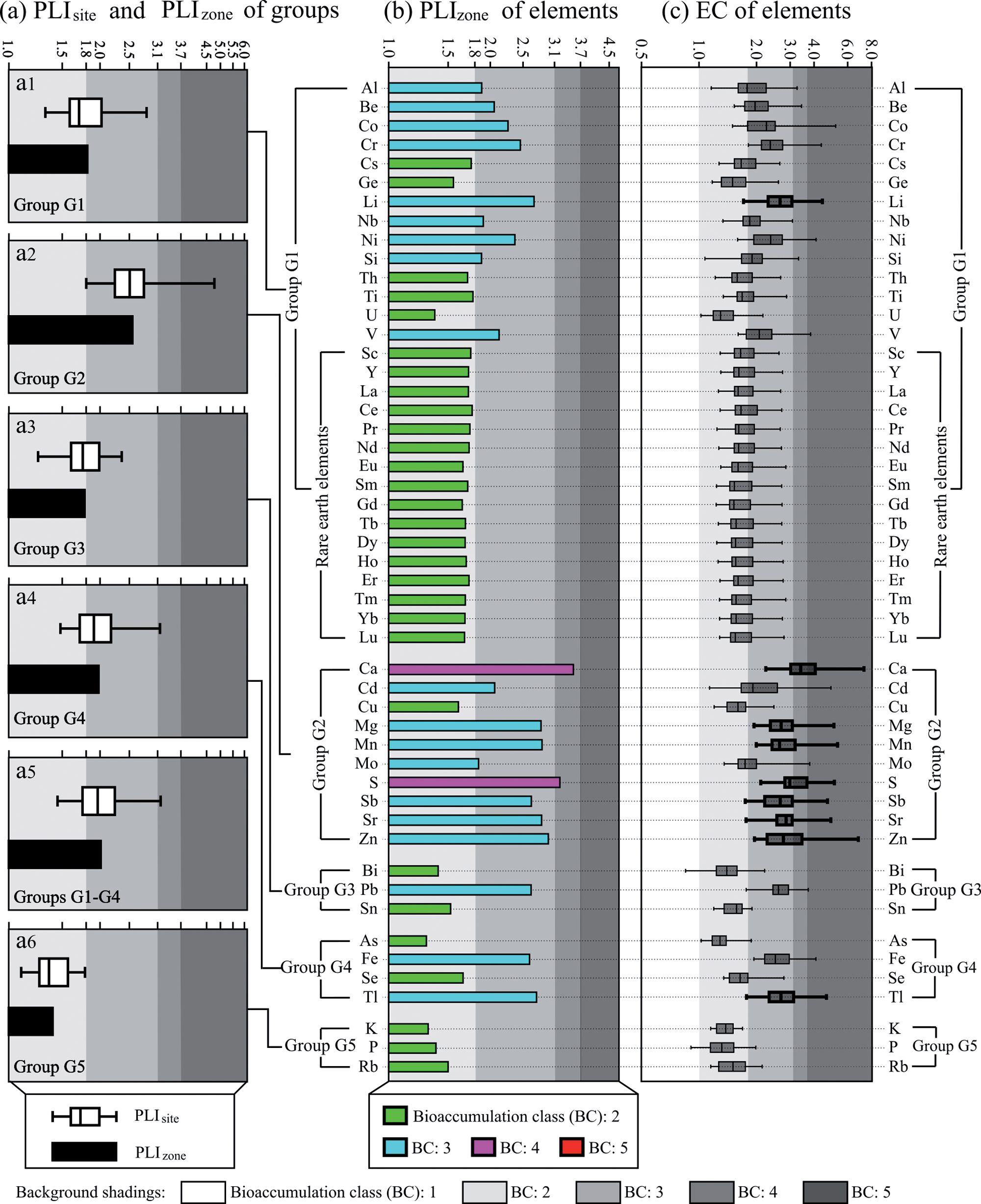
See Fig. 2a-c for the EC and PLI of the elements in all 5 groups. According to the results, PLIzone of G1, G2, and G4 belongs to the bioaccumulation of Class 3. PLIzone of G3 and G5 belongs to the bioaccumulation of Class 2. The PLIzone of the combined groups G1-4 belongs to the bioaccumulation of Class 3.
PLIsite of G2 belongs to the bioaccumulation of Class 3 to 5 at all the exposure sites. PLIsite of G5 belongs to the bioaccumulation of Class 2 at all the exposure sites. PLIsite of G1, G3, and G4 belongs to the bioaccumulation of Class 2 and 3 at most of the exposure sites. PLIsite of the combined group G1-4 belongs to the bioaccumulation of Class 2 and 3 at most of the exposure sites.
At the level of elements, both PLIzone and EC of Ca and S are far higher than those of other elements, and their PLIzone belongs to the bioaccumulation of Class 4, and their EC belongs to the bioaccumulation of Class 4 and 5 at ≥50% of the exposure sites (Fig. 2b-c). In addition, the EC of 7 elements (Li, Mg, Mn, Sb, Sr, Zn, and Tl) belongs to the bioaccumulation of Class 4 and 5 at ≥25% of the exposure sites (Fig. 2c).
Kriging Analysis
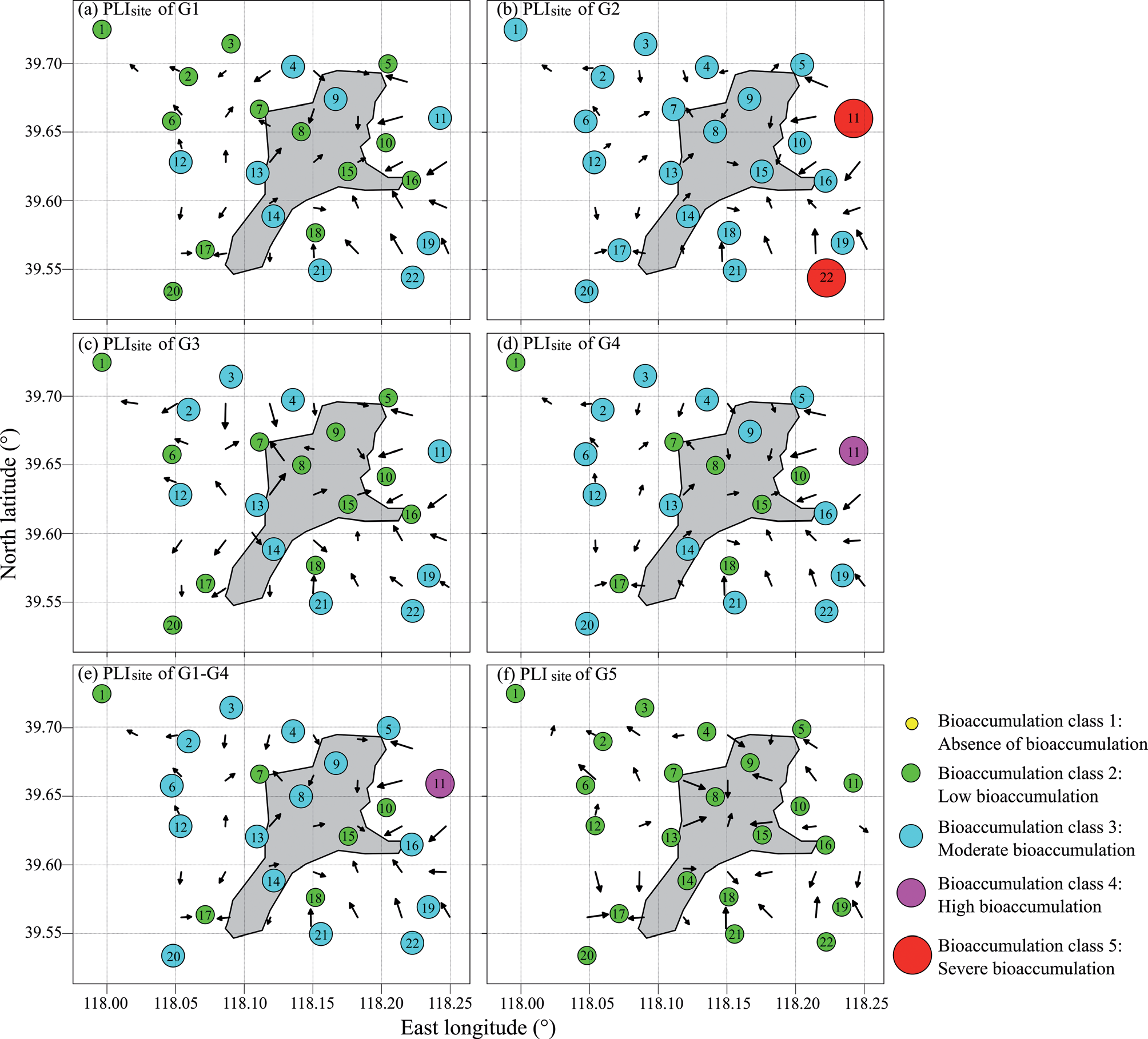
See Fig. 3a-f for the results of Kriging analysis on the element group PLIsite. According to the results, the PLIsite of the 5 groups shows a similar spatial pattern, characterized by a decreasing trend from east to west and from rural to urban areas. PLIsite of G2 belongs to the bioaccumulation of Class 5 at exposure sites 11 and 22 and the bioaccumulation of Class 3 at the remaining 20 exposure sites (Fig. 3b).
Discussion
Elements not Suitable for Biomonitoring
Our results have proved the conclusion of previous studies that the environmental availability of some elements is not always effectively reflected by active biomonitoring using lichens [39, 40]. In our study, the bioaccumulation of 4 out of 51 elements (Ag, K, P, and Rb) in RSI is not an appropriate indicator of atmospheric deposition. Firstly, the exposure concentration of Ag is not significantly different from the background concentration on a regional scale (Table 1) and has no significant difference with the background at 10 of 22 exposure sites (Table 1; independent-samples T test, p≤0.05), which contradicts the result that atmospheric suspended particulate matters in the exposure area were higher than those in the background area during the experiment (Fig. 1e).
K, P, and Rb are classified into G5 alone, which is defined as the group of nutrient elements not suitable for biomonitoring. The exposure concentration of G5 elements is significantly higher than the background value on a regional scale (Table 1) and at most of the exposure sites (Table 1; independent-samples T test, p≤0.05). However, these elements have lower EC values, PLI values, and bioaccumulation levels than the remaining 47 elements (Fig. 2). The lower bioaccumulation level of these nutrient elements may be related to the higher background concentration induced by physiological regulation because lichens in the background area with a lower level of atmospheric deposition will selectively absorb and retain K and P [41]. As a result, the bioaccumulation class is underestimated, even though the exposed thalli also accumulated K and P (Table 1). In fact, previous studies have also pointed out that the response of nutrient element concentration in lichen to atmospheric element deposition is different from or even opposite to that of non-nutrient elements. Bennett and Wetmore pointed out that the nutrients and stress elements in lichens show different concentration responses to atmospheric deposition, both spatially and temporally [42]. Bennett and Wright discovered that the spatial pattern of K and P in lichens is opposite to that of the pollutants Cu, Pb, and Zn [43]. Adams and Gottardo also discovered this fact [35]. Wu et al. discovered that concentrations of the elements associated with traffic pollution in two lichens increase with decreasing road distance, but K and P concentrations remain unchanged [44]. Gao et al. discovered that the concentration of nutrients (K and P) and the elements with less significance of physiology have opposite spatial distributions in different parts of lichen [45]. Therefore, active biomonitoring using RSI may greatly underestimate the atmospheric deposition of K and P. Otherwise, the threshold of bioaccumulation class must be lowered for K And P to Compensate for Such Underestimation.
Fig. 3.
Kriging analysis of PLIsite of element groups. Note: The shaded part represents the urban area while other parts represent suburban and rural areas. The black arrow indicates a decreasing trend of PLIsite.
We recommend RSI to monitor the 47 elements from G1 to G4 because the exposure concentration of these elements is significantly higher than that of the background concentration on both regional and local scales (Table 1). This result is consistent with the variation of atmospheric pollutant concentration during the experiment (Fig. 1e).
Element Source
According to the PCA results, 50 elements (excluding Ag) are divided into 4 PCs and 5 element groups (Table 2). The G5 belongs to nutrients, as mentioned above, while the other 4 groups are of crustal and/or atmospheric origin induced by human activities in Tangshan.
The G1 elements are mainly of crustal origin (Table 2; Fig. 2). Sixteen rare earth elements are regarded as tracer elements of crustal origin in many relevant studies [24, 46-48]. Al and Si are rock-forming elements. The elements in this group may result from the deposition of soil particulates induced by human activities.
The G2 (Ca, Cd, Cu, Mg, Mn, Mo, S, Sb, Sr, and Zn) and G3 (Bi, Pb, and Sn) elements are mainly of atmospheric origin induced by human activities. The G2 elements are pollutants emitted from diverse human activities, including industrial, traffic, and household activities. For example, S is the most common product of fossil fuel combustion. In the heating period, industrial and household activities with coal as the fuel emit a large amount of SO2 into the atmosphere [1], which is the main pollutant of haze in the North China Plain [2]. This situation is also confirmed by the fact that the SO2 concentration in the exposure area is higher than that in the background area (Fig. 1e). Ca is regarded as an important tracer of dust pollution in the cement industry [49]. The other 8 elements in G2 are often emitted by traffic and other industrial activities, such as metal smelting, alloy processing, and power generation [8, 10, 36, 50, 51]. For example, Mo, Sb, and Sr are the special tracers of vehicle mechanical consumption [52, 53]. The G3 elements can be emitted in large amounts from the alloy industry and manufacturing industry. Bi-Pb-Sn are frequently used as solder alloys in mechanical and electronic manufacturing and as cryogenic coolants in the power industry [54].
The bioaccumulation of G4 elements (As, Fe, Se, and Tl) in RSI is affected by both crustal and atmospheric sources because these elements have moderate factor loadings (Table 2) on multiple principal components. For example, Fe has a moderate factor loading on PC1 (0.59), PC2 (0.39) and PC3 (0.46; Table 2), which is consistent with the consensus that Fe is an indicator element of crustal input [55] and a marker of emissions from the iron and steel industry [56]. Tl has a moderate factor loading on PC1 (0.62), PC2 (0.57) and PC3 (0.46; Table 2), which is consistent with the consensus that Tl is often of crustal origin [57], an industrial pollutant [18], and an indicator element of coal combustion [52].
Bioaccumulation Level
Our results indicate that the level of atmospheric element deposition in Tangshan is high, though we used an interpretive scale that may overestimate the bioaccumulation level. On a regional scale, the overall bioaccumulation in RSI is moderate bioaccumulation, according to the PLIzone of the combined groups of G1-4 (Fig. 2a5). This result coincides with the fact that the city has frequent industrial and agricultural activities, a developed transportation network, and coal combustion for heating in winter.
Atmospheric deposition of G2 elements is the most noteworthy because this atmospheric group has higher PLIzone and more exposure sites with moderate bioaccumulation (Fig. 2a) than the other 3 groups. As mentioned above, G2 elements are associated with various human activities, such as industrial, traffic, and household activities. The iron and steel industry is a major industry in Tangshan. Energy, the chemical industry, building materials, and manufacturing are developed here. This industrial structure is the primary reason that the G2 elements have a higher bioaccumulation level than the other groups. Therefore, we suggest that the importance of the G2 elements should be emphasized in active lichen biomonitoring of atmospheric deposition in North China cities.
At the level of elements, attention should be paid to the emissions of Ca and S because the bioaccumulation of the two elements is high on a regional level, which is far higher than that of other elements (Fig. 2b). Attention should also be paid to the emissions of 7 elements (Li, Mg, Mn, Sb, Sr, Zn, and Tl) because the bioaccumulation of these elements is high and severe at ≥25% of the exposure sites (Fig. 2c).
Spatial Pattern
The Kriging analysis result of PLIsite for the combined groups G1-4 (Fig. 3e) shows an apparent trend of decreasing atmospheric element deposition from east to west and from rural areas to urban areas. And this trend has been observed in all 5 groups (Fig. 3a-d, f). This trend is related to the spatial distribution of industrial facilities, agricultural activities, and coal combustion in the study area. Plant facilities are mostly distributed in the east and in rural and suburban areas (Fig. 1c). Agricultural activities are frequent, and coal is burned for heating in rural areas in winter. The atmospheric group (G2) has the highest PLIsite at two exposure sites (11 and 22) in the east (Fig. 3b), indicating a strong local impact of industrial, agricultural, and coal-burning emissions in suburban and rural areas in the east on atmospheric element composition. All the groups have a low PLIsite at sampling point 1 in the west because this sampling point is close to the airport (Fig. 1c), where industrial activities are restricted.
In general, the atmospheric pollution control measures taken by Tangshan have achieved a positive effect in recent years (PLIzone of the combined G1-4 belongs to moderate bioaccumulation). However, further attention should be paid to anthropogenic emissions, especially in rural areas.
Conclusions
We validated RSI as a good active biomonitor for 47 elements but not for Ag, K, P, and Rb in North China cities for the first time and highlighted the importance of the atmospheric G2 metals (especially Ca, S, Mg, Mn, Sb, Sr, and Zn) in active lichen biomonitoring techniques in these cities. Affected by the industrial structure dominated by the iron and steel industry, the overall bioaccumulation of 47 elements belonging to 4 groups is moderate in the study area. Attention should be paid to the atmospheric group G2, which is of high to severe bioaccumulation at ≥25% of the exposure sites. The PLIsite of all groups shows a similar trend of decreasing from east to west and from rural areas to urban areas, apparently resulting from frequent industrial, agricultural, and coal-burning activities in the east and in rural areas. For the above reasons, sustained attention should be paid to anthropogenic emissions in rural areas, especially those from industrial and coal burning activities.