

Introduction
In the context of the global greenhouse effect, the United Nations General Assembly put forward two crucial international climate change agreements, the Kyoto Protocol and the Paris Agreement, in 1997 and 2015, respectively, to promote carbon emission reduction utilizing market instruments [1]. The European carbon market was officially launched in 2005. As the world’s most mature carbon trading market, it plays a vital role in carbon emission reduction activities. China, the largest developing country, has been actively assuming the responsibility of a significant country in environmental governance. Since 2013, China has set up eight regional carbon trading pilots, and in 2020, at the 75th United Nations General Assembly, formally proposed the goal of “peaking carbon dioxide emissions before 2030 and achieving carbon neutrality before 2060” [2]. On July 16, 2021, China officially launched the trading activities of the national carbon market, driving the development of the domestic carbon market into a new phase. Carbon price forecasting plays a pivotal role in the market trading system. From a macro perspective, the carbon price directly reflects changes in the supply and demand of carbon emission rights in the market. Accurate forecasting of the carbon price can, on the one hand, give full play to the role of price regulation to adjust the allocation of market resources. On the other hand, it can also provide information to establish carbon market management policies [3]. From a micro perspective, carbon price forecasting can assist enterprises in understanding the future development trend of the market to rationally formulate carbon trading strategies to improve their profit level under the premise of completing compliance.
With the in-depth study of carbon price forecasting, a large number of forecasting methods have been accumulated in this field, which can be categorized into three major groups: econometric, artificial intelligence, and hybrid model forecasting. The first category, the econometric method, involves discovering the dynamic laws embedded in natural economic or measurement systems by establishing stochastic equations to describe the quantitative characteristics of real problems [4]. It includes the ARIMA (autoregressive integrated moving average) model [5], ARMA (autoregressive moving average) model [6], GARCH (generalized autoregressive conditional heteroscedasticity) model [7], VAR (vector autoregressive) model [8], and so forth., all of which have achieved good forecasting results in the regional carbon markets they have studied. The second category is artificial intelligence methods. Artificial intelligence models have gained wide application in recent years due to their strong generalization ability and ability to capture nonlinear relationships [3]. In early research, scholars worked on combining various artificial intelligence models such as BPNN (backpropagation neural network) [9], ELM (extreme learning machine) [10], and LSSVR (least squares support vector regression) [11] with different optimization algorithms to forecast carbon prices. In subsequent research, RNN (recurrent neural network models) such as the LSTM (long short-term memory) neural network [12] and the GRU (gated recurrent unit) neural network [13] stand out among all artificial intelligence models with their unique memory functions and have become one of the most frequently used forecasting models. The third category, hybrid model forecasting methods, arose from the need to cope with the complexity and variability of carbon price series [14]. Among the hybrid model forecasting methods, the decomposition integration strategy, which advocates the decomposition of the carbon price series before forecasting, has recently become one of the mainstream research methods in the field. It reduces the complexity of the original series as well as the requirements of the forecasting model [15]. The main signal decomposition methods used in this strategy are the EMD (empirical mode decomposition) model [16], the EEMD (ensemble empirical mode decomposition) model [17], the VMD (variational mode decomposition) model [18], the CEEMD (complementary ensemble empirical mode decomposition) model [19], and the CEEMDAN (complete ensemble empirical mode decomposition with adaptive noise) model [20].
Fluctuating carbon prices are highly susceptible to the influence of the external environment, so increasing the consideration of external influencing factors can improve the accuracy of the forecast. The influencing factors considered by scholars can be roughly divided into two categories, namely structural factors and non-structural factors. Structural factors mainly include energy prices, the economic situation, international carbon prices, and the environment. Fossil energy prices, such as coal, oil, and natural gas, influence supply and demand in energy markets, which are closely linked to carbon emissions and prices [21]. The economic situation corresponds to the activity of enterprises, which can indirectly affect their demand for carbon allowances [22]. The influence of the international carbon price, represented by the EU carbon price, on domestic carbon prices stems from the strong information spillover effect of this mature trading market [23]. Environmental factors, such as air quality and extreme temperatures, affect carbon prices through regulatory intensity and energy consumption, respectively [24]. Non-structural factors mainly refer to the Baidu search index, which is widely used in China. It reflects, to some extent, changes in investors’ behavior and their interest in carbon markets [25].
Carbon price forecasting has accumulated a wealth of research results, but some things still could be improved. Regarding research content, most of the literature on carbon price forecasting only focuses on describing the performance of the forecasting models but neglects the correlation analysis of forecasting results. In terms of the forecasting models, although LSTM and GRU models have excellent memory functions, they can only capture forward time series information, which quickly causes information loss and affects forecasting accuracy. Based on the above considerations, this paper proposes a hybrid forecasting model integrating influencing factor screening, signal decomposition, and carbon price forecasting. Initially, the LASSO (least absolute shrinkage and selection operator) algorithm is used to screen out the main external influencing factors from aspects of the foreign carbon price, energy price, macroeconomics, market exchange rate, industrial development, and environment. They are used as model inputs, along with the carbon price, to participate in forecasting. Secondly, the original carbon price series is decomposed with the VMD model and reconstructed according to SE (sample entropy). Then, the BIGRU model, which can extract information from both forward and reverse directions, is selected to forecast the reconstructed series combined with the main influencing factors and the final forecasting values are obtained by integrating their forecasting results. Finally, an analysis of the reasons for changes in trends in forecasting results is provided.
The features and innovations of this paper are mainly in the following two aspects: First, the VMD-BIGRU model, which has been widely used in the forecasting fields of crude oil price, wind power, and gold futures price, is applied to the field of carbon price forecasting, and its superiority in this forecasting task is confirmed, which contributes to the further in-depth development and application of the BIGRU model in this field. Second, after the end of the forecasting process, combined with the actual development of the market and the changes of external influencing factors, the trend analysis of the carbon price forecasting results is carried out, and the reasons for changes in the trend are expounded. Based on this, we make reasonable forecasts of future changes in carbon prices outside the sample.
Experimental Procedures
This paper proposes a hybrid carbon price forecasting model integrating influencing factor screening and decomposition integration, including the LASSO algorithm for influencing factor screening, the VMD model for decomposition, the BIGRU model for forecasting, and the evaluation indicators, as well as the DM (Diebold-Mariano) test for comparison of forecasting effects of models, and takes the carbon price in Hubei as the research object for forecasting.
Framework for the Hybrid Carbon Price Forecasting Model
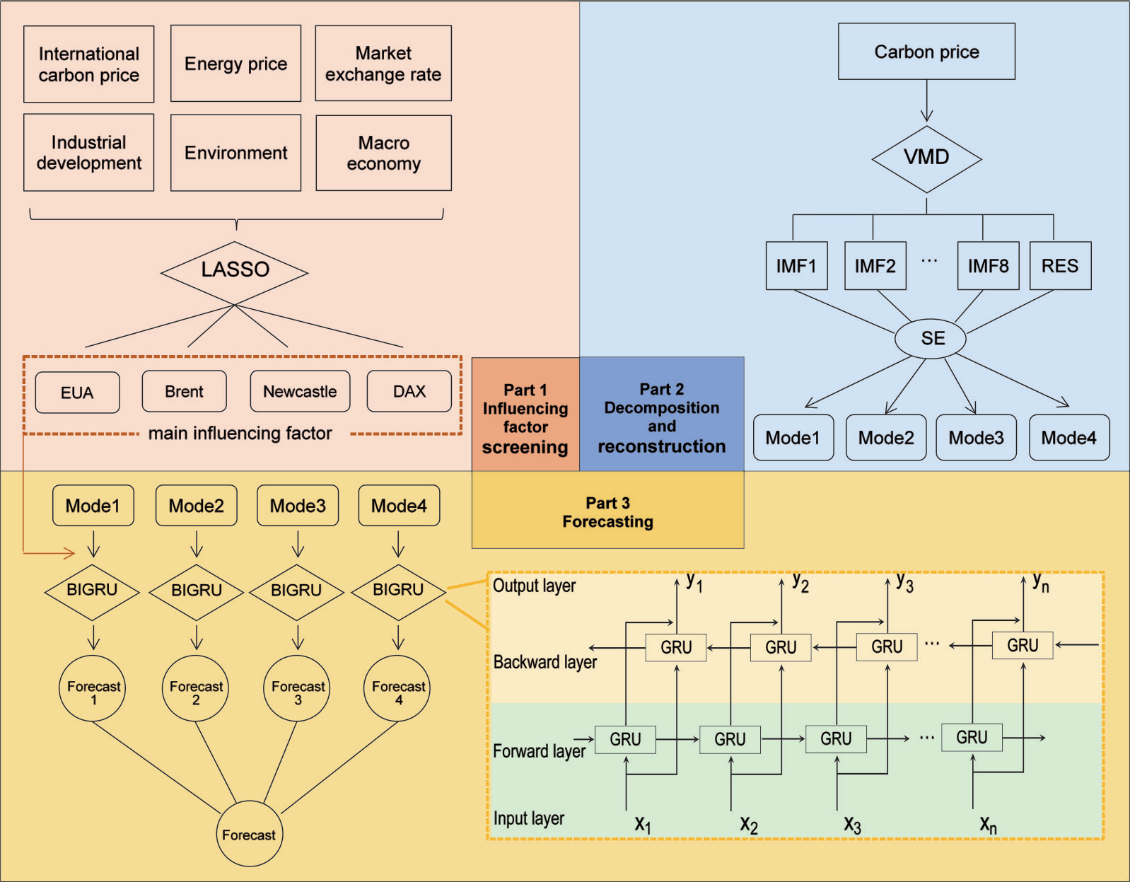
The structure of the hybrid carbon price forecasting model used in this paper is shown in Fig. 1 and contains three main components. The first part screens the influencing factors of the carbon price. The LASSO algorithm is used to screen out the main influencing factors with a high degree of correlation with carbon prices from six aspects: international carbon price, energy price, macroeconomics, market exchange rate, industrial development, and environment. The second part is the decomposition and reconstruction of the carbon price series. To reduce its complexity, the original carbon price series is decomposed into several IMFs (intrinsic mode functions) with different data characteristics by the VMD model and reconstructed into a new series named Mode according to the SE value of each IMF. The third part is carbon price forecasting. The BIGRU model extracts essential information from the series and combines the screened influencing factors to forecast each Mode series separately. Then, their forecasting results are linearly summed to get the final forecasting value.
LASSO Algorithm
The LASSO algorithm was proposed by Robert Tibshirani in 1996 and is essentially a shrinkage estimation method [26]. It achieves indicator screening and model simplification by adding the L1 norm to the objective function of traditional least squares estimation to impose penalties on the model’s coefficients and compress the coefficients of unimportant independent variables to zero. The specific expression is:
Where argmin is the function to find the minimum value of the parameter, yi is the vector of dependent variables, xij is the matrix of independent variables, βj is the vector of coefficients, and λ is the regularization coefficient. λ determines the penalization strength of the model; the larger its value, the stronger the model penalizes, and the fewer variables are screened out.
VMD Model
In 2014, Dragomiretskiy and Zosso applied the Wiener filter to multiple adaptive bands. They proposed a fully non-recursive variational modal decomposition model, demonstrating strong robustness in sampling and denoising [27]. The key to this decomposition method is to construct and solve variational models [28]. It decomposes the original signal into specified k mode functions with finite bandwidth by iteratively searching for an optimal solution, and their superposition can reproduce the original signal completely. The detailed decomposition steps of the model are as follows:
Step 1: Compute the analytic signal of the mode function uk (t) by the Hilbert transform.
Step 2: Calculate the center frequency of each mode function by adjusting the exponential term, and then modulate the spectrum of uk (t) to the fundamental frequency band.
Step 3: Construct the variational constraint problem to find the mode function when the sum of the bandwidths of their center frequencies is minimized.
Step 4: Introduce the Lagrange multiplication operators λ(t) with a quadratic penalty factor α to transform the constraint equation into an unconstrained one.
Step 5: Solve the variational problem constructed above by applying the multiplicative alternating direction method. The corresponding calculation steps can be found in the reference [29].
BIGRU Model
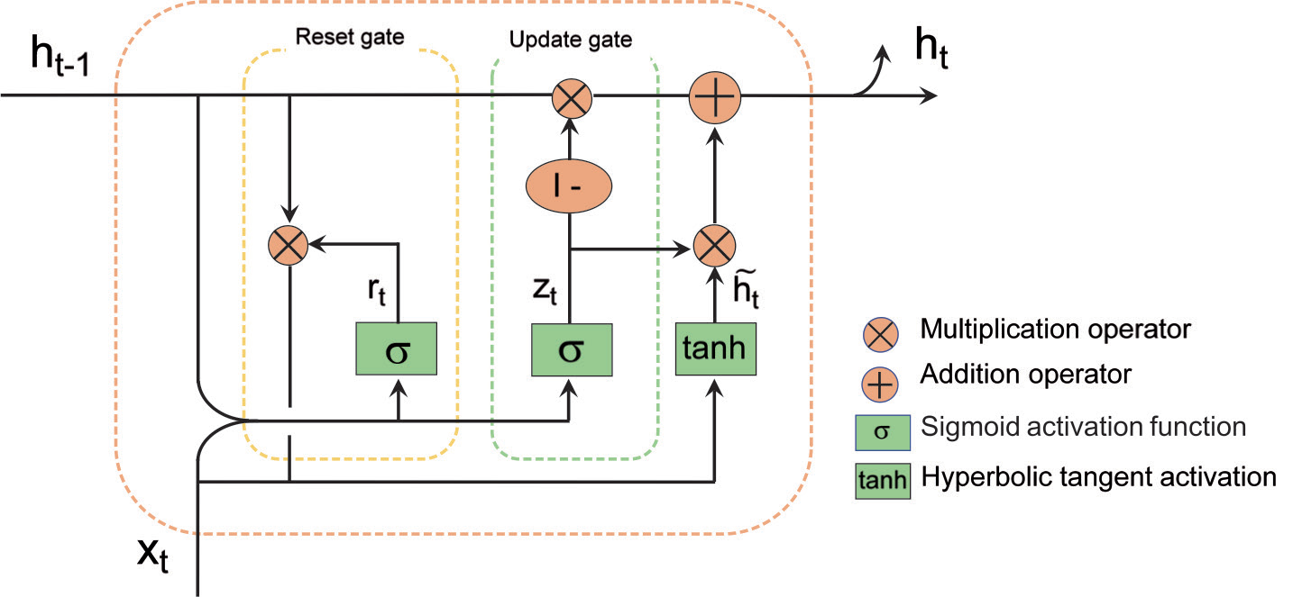
The basic unit structure of the BIGRU model consists of two independent GRU units connected. The GRU model is a special kind of RNN that not only solves the short-term memory problem of traditional RNN but also overcomes gradient vanishing. As a simplified version of the LSTM model, only two gating structures, the update and reset gates, are included in the GRU. The update gate controls the extent to which the previous moment’s memorized information is brought into the current state. In contrast, the reset gate determines how much the new input information is combined with the previous moment’s memorized information [30]. The specific structure is shown in Fig. 2.
Equations (2)-(5) show the corresponding internal calculations.
The update gate:
The reset gate:
The reset gate state vector rt is combined with ht–1 and xt to compute the state vector of the candidate hidden layer:
Finally, the hidden layer state vector at the current moment is computed by combining ht–1 with
Where rt, zt are the state vectors of the reset gate and the update gate at the moment t, respectively. σ is the activation function. Wr, Wz, and
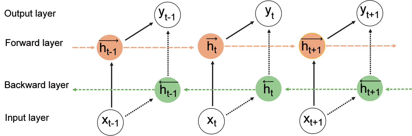
The current level of carbon prices in the market responds to historical carbon prices and is also the basis for future carbon price setting. Therefore, it has a two-way correlation. However, GRU can only transfer series information in one direction; if the length of the series is considerable, a large quantity of information will be lost in the final state, which affects the learning situation of the model and then reduces the forecasting accuracy. The BIGRU model chosen in this paper connects the two GRU hidden layers in the forward and reverse directions, which allows it to take both the past and future valuable data messages into account to ensure the completeness of the learning information. The basic structure of the model is shown in Fig. 3.
The internal formulas are shown in Equations (6)-(8).
The forward output sequence of the GRU hidden layer after the preceding iteration is:
Similarly, the backward output sequence of the GRU hidden layer is:
The final output sequence of the BIGRU model is represented as:
where the G( ) function represents a nonlinear transformation of the model inputs, that encodes the degradation metrics into the corresponding GRU hidden states. wt, vt are the weights of the forward hidden layer state
Criteria for Assessing the Forecasting Effect of the Models
This paper uses traditional evaluation indicators and the significance test of differences to measure the effect of different forecasting methods. In terms of traditional evaluation indicators, six indicators, including MAE (mean absolute error), MSE (mean square error), RMSE (root mean square error), MAPE (mean absolute percentage error), R2 (coefficient of determination), and Dstat (directional change statistics), are selected from the perspectives of forecasting error, goodness of fit of the model, and directional accuracy. The first four indicators in the forecasting error category are inversely related to the forecasting effect, while R2 and Dstat are positively related. Regarding the significance test of differences, we introduce the DM test proposed by Diebold and Mariano. The original hypothesis of the test is that two models possess the same forecasting accuracy. If the p-value is small, the original hypothesis can be rejected, indicating that the difference in forecasting accuracy between the two models is significant. As for the superiority or inferiority of forecasting, the effect between them can be judged according to the positive or negative sign of the DM value. Specific arithmetic steps are detailed in the literature [31].
Empirical Research
The empirical part of the study begins with screening for external influencing factors, decomposition and reconstruction of the normalized carbon price series, and then forecasting the reconstructed series in combination with the main influencing factors.
Data Sources and Preprocessing
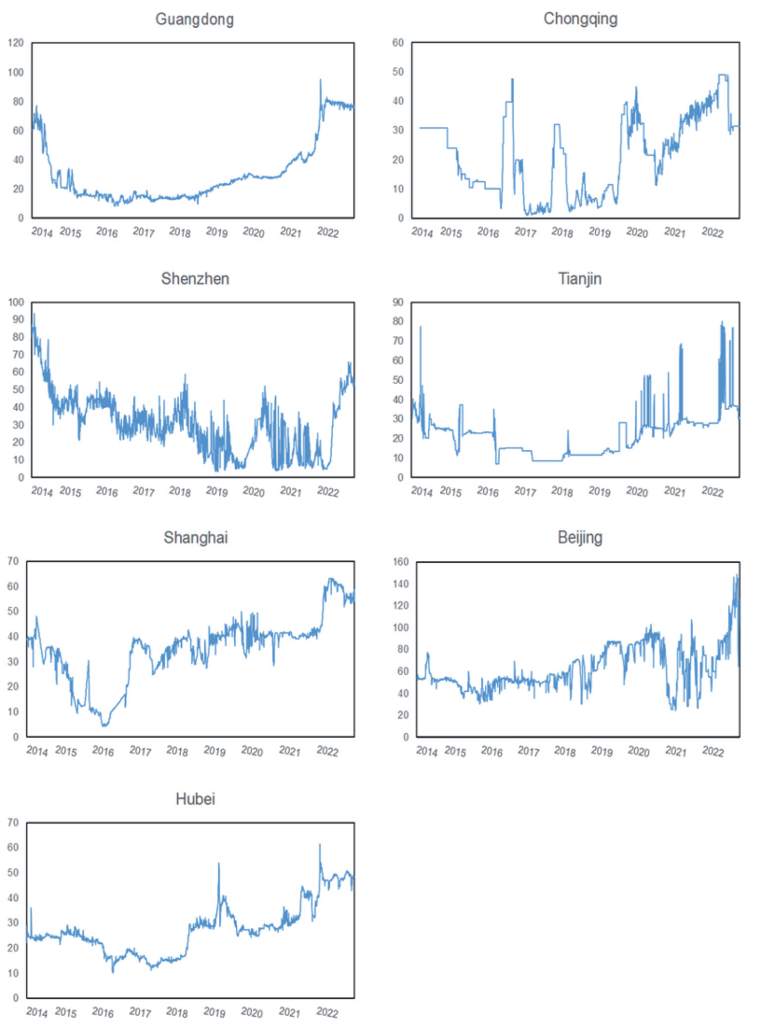
Since 2013, China has established eight carbon trading pilots, and the changes in carbon prices in each province are shown in Fig. 4. Carbon prices in Chongqing, Shenzhen, Tianjin, Shanghai, and Beijing all fluctuated dramatically and frequently. Although carbon prices in Guangdong have had a relatively smooth trend without frequent fluctuations, there were significant decreases and increases in July 2014 and November 2021, respectively. Compared to other regions, the carbon price in Hubei has changed more gently and has maintained an overall stable trend of fluctuating upward over the years. In addition, as the regional carbon market with the largest carbon trading volume and turnover, the trading entities of the Hubei carbon market are not limited to the Hubei region, and the trading activity of this market has always been in a leading position. Therefore, we take the closing price in trading days of carbon allowances in the Hubei carbon market as the research object. As shown in Fig. 5, the sample interval is from April 2, 2014, to December 31, 2022.
In addition to the historical data on carbon prices, we comprehensively consider the outside world’s influence on them and select 16 exogenous variables to assist in forecasting the carbon price. The selection of variables is shown in Table 1. The data are obtained from Wind, except for the average daily temperature in Wuhan, which is obtained from the Meteorological Data Center. After removing missing data, there are 1789 sets of standard data intervals for all variables; the first 1689 sets are used as training sets, and the last 100 sets are test sets.
According to the results of the descriptive statistics in Table 2, there are apparent dimensional gaps among the 17 variables. All of them are uniformly normalized to avoid any influence on the subsequent study. From the ADF test results of the carbon price in Fig. 5, it is clear that the original carbon price series has a high degree of non-stationarity and needs to be decomposed in the next step to realize accurate forecasting.
Screening of Influencing Factors in the Carbon Price
In this paper, 16 variables are selected to represent the influence of external factors on carbon prices from six aspects: foreign carbon price, energy price, market exchange rate, macroeconomics, industrial development, and environment. As shown in Table 3, the average variance inflation factor is greater than 10, which implies the existence of solid multicollinearity, so we applied the LASSO algorithm, which can deal with this problem efficiently, to screen factors influencing the carbon price.
The coefficient of the penalty term, λ, is the most critical hyperparameter in the LASSO algorithm and controls the complexity of the function. We apply the ten-fold cross-validation to determine the optimal value of it as 0.000587 and build the model based on this. The function in the model is then solved by the coordinate descent method to obtain the weight coefficient of each variable, which represents the degree of its influence on the carbon price. As shown in Fig. 6, the coefficients of a total of 9 variables are not compressed to 0 after screening, but 5 are less than 0.1, which has a negligible impact on the carbon price. To simplify the forecasting model’s structure, we choose the top 4 variables in terms of importance, EUA, Brent, DAX, and Newcastle, to participate in the forecast along with the carbon price as model inputs.
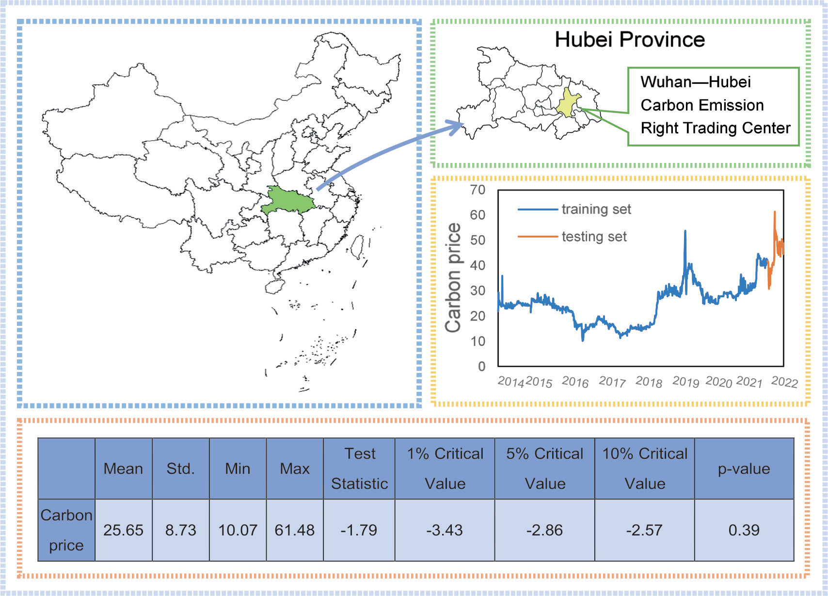
Table 1.
Influencing factors of the carbon price.
Table 2.
Descriptive statistics of variables.
Table 3.
Variance inflation factors of variables.
| Variable | VIF |
|---|---|
| SP500 | 57.89 |
| WTI | 56.72 |
| Brent | 53.23 |
| Average | 50.48 |
| Low | 26.64 |
| EUA | 25.4 |
| Newcastle | 21.64 |
| ARA | 20.45 |
| High | 19.32 |
| CSI300 | 18.05 |
| DAX | 12.46 |
| Industry | 11.64 |
| NYMEX | 6.65 |
| Euro | 5.17 |
| Dollar | 3.05 |
| AQI | 1.33 |
| Mean value | 24.38 |
The weight coefficient of EUA is as high as 0.86, which is the most important influencing factor of the carbon price in Hubei. Due to the late start of the carbon market and the lack of corresponding management experience in China, the European carbon market, which is the most mature market, has been used as a reference for the design of the trading system and the management of the domestic market. Coupled with the fact that traders in the Hubei carbon market include a large number of overseas institutions and individual investors in addition to emission-control enterprises and that the level of foreign carbon prices influences the investment decisions of these market participants, price changes in the EUA can have a significant impact on the carbon price in Hubei. DAX, as one of the key indices of the global securities market, represents the economic development of the European Union. China participates in international carbon trading mainly through the CDM (clean development mechanism) projects, and the primary demand side of these projects is the European Union countries, so there is a correlation to some extent between their economic level and the carbon price in Hubei, which has the largest trading volume in China. In terms of energy prices, although both Newcastle and Brent influence the carbon price level in Hubei, Newcastle has a slightly higher degree of importance than Brent, which is determined by the structure of energy consumption in Hubei Province. As a central industrial province in China, its industrial structure favors heavy industry, so coal and oil are the main energy sources it consumes. Based on its energy consumption trends from 2001 to 2021, coal consumption is much larger than oil, which, coupled with coal’s higher carbon emission factor, makes the carbon price in Hubei more closely linked to coal than oil’s price.
Decomposition and Reconstruction of the Carbon Price Series
Decomposing the carbon price series can reduce its randomness and nonstationarity [32]. We determine the optimal value of the decomposition number K in the VMD model by observing the central frequency of IMFs. As seen from Table 4, when the decomposition number is less than 8, the center frequency of the IMF with the lowest frequency varies with the decomposition number, indicating that the decomposition is insufficient, which easily causes the phenomenon of modal aliasing. When the decomposition number exceeds 8, its center frequency stabilizes significantly. If the decomposition continues, it will easily lead to excessive decomposition. On the one hand, the workload will be increased in vain, and the forecasting efficiency will be reduced. On the other hand, it will be easy to include useless variables, which affect the forecasting model’s ability to extract data features. Therefore, the value of K is set to 8, and the penalty factor α takes the value of 2000.
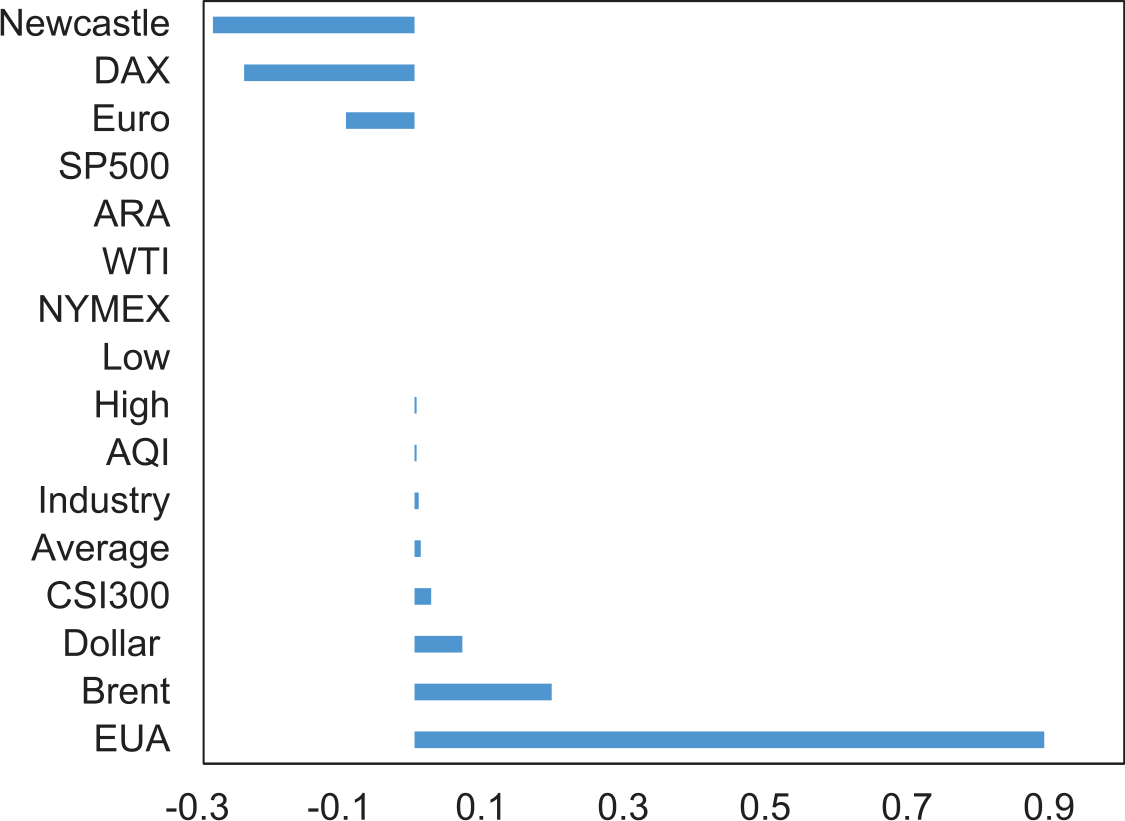
Table 4.
Center frequency of each IMF under different decomposition numbers.
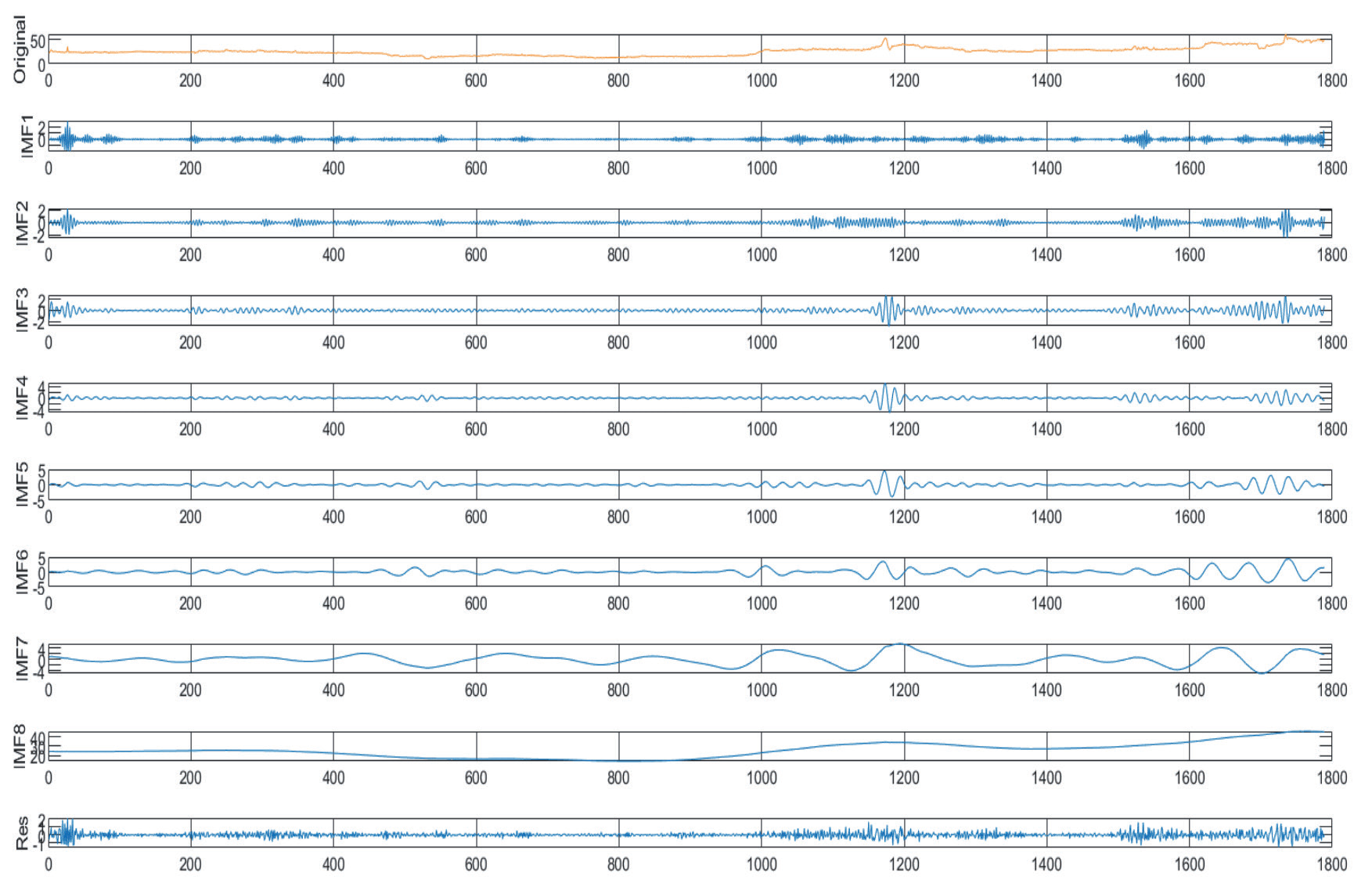
The original input series and the final decomposition result of the VMD model are shown in Fig. 7. Due to the large number of IMFs after decomposition, to simplify the forecasting process, we reconstruct them with SE, which measures the complexity of time series, and name the new series Mode. The SE values and reconstruction results for each IMF are presented in Fig. 8. Mode 1 and Mode 2 record the fluctuation of the carbon price in Hubei, while Mode 3, which has the lowest complexity, strips out the high-frequency fluctuation of the carbon price and retains the overall trend of the series.
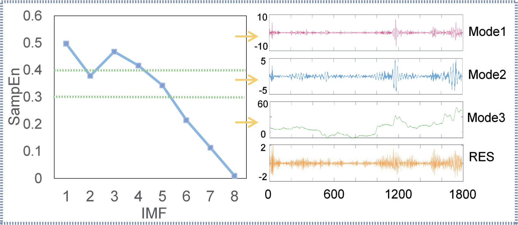
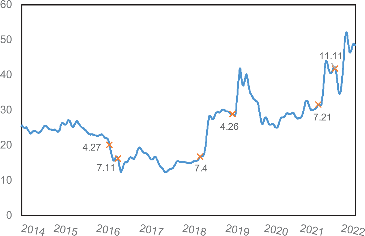
As can be seen from Mode 3 in Fig. 9, the carbon price in Hubei shows a basic trend of decreasing and then increasing. Initially, the carbon allowance auction held before the opening of the Hubei carbon market played a role in price discovery, so the carbon price in Hubei was maintained at 20 yuan from 2014 to the first half of 2015. In the second half of 2015, the domestic economy downturned and commodity prices continued to weaken, coupled with the severe situation of industrial enterprises in Hubei to reduce overcapacity. Hence, the carbon price began to show a downward trend. It then spent the next two years at a low price point of 15 yuan due to the low EUA and rising Newcastle. It was not until 2018 when Hubei lowered its market entry threshold, coupled with the launch of the national carbon market, which made the Hubei carbon market increasingly active, that carbon prices began to appear and generally maintained a growth trend.
The fluctuation trend of the carbon price in Hubei contains six mutation points: April 27, 2016; July 11, 2016; July 4, 2018; April 26, 2019; July 21, 2021; and November 11, 2021. The launch of forward quota products in the Hubei carbon market on April 27, 2016, transferred a large number of spot transactions, causing the first precipitous drop in carbon prices. On July 11 of the same year, due to the sudden announcement of the compliance deadline in the Hubei market, enterprises with only four days to deal with their remaining allowances chose to sell their excess allowances at a low price before the government collected them. However, the market could not take over all allowances, which led to a sudden drop in carbon prices by nearly 40%. After that, the government urgently adjusted the bargaining range and limited the extent of the reduction to make a slight recovery. On July 4, 2018, the market was in the compliance phase, and more enterprises started to participate in carbon trading owing to the lowering of the entry threshold. Coupled with the impact of the significant increase in EUA, the Hubei carbon price gradually climbed to a price range of 25-30 yuan. On April 26, 2019, as the compliance period approached, market activity increased, making the carbon price fluctuate significantly. On July 21, 2021, with the launch of the national carbon market, people’s attention to the Hubei carbon market increased, and the number of institutions and individuals who opened accounts in the market soared. Afterward, market speculation was at an all-time high, increasing the carbon price by more than 10 yuan. On November 11, 2021, the market was informed in advance of the base price for the allowance auction, and as a result, high carbon prices suffered a brief period of suppression.
Carbon Price Forecasting
We take Modes and four main influencing factors screened out together as model inputs and used the BIGRU model to forecast Mode 1-4 3-5 times. Then, the best results are selected for saving. Finally, we linearly sum up the forecasting results of each Mode to get the final forecasting value. In terms of model training, this paper chooses the Adam optimizer, which has the advantages of fast convergence and small memory capacity, to optimize the training process to reduce the number of iterations required to obtain the optimal parameters and accelerate the optimization process [33]. In the iterative optimization of parameters using the gradient descent algorithm, the MSE function is chosen as the loss function, considering the dynamic variation of the gradient value. The remaining essential parameter settings of the model are shown in Table 5.
Results and Discussion
Analysis of the Carbon Price Forecasting Results and the Reasons for Changes in Its Trend
The hybrid carbon price forecasting model VMD-BIGRU adopts the forecasting idea of decomposition and integration to forecast the carbon price in Hubei. Fig. 10 shows the final forecasting result and its trend changes.
The forecasting results of the carbon price can be categorized into three phases based on their respective trends: the early phase, the middle phase, and the late phase. In the early phase, along with the establishment of China Carbon Emissions Registration and Clearing Co., LTD., the market activity in Hubei increased. Coupled with the combined influence of external factors such as the continuously rising Brent and EUA as well as the declining DAX, the carbon price has mainly shown a fluctuating upward trend. In the middle phase, there was a sharp fluctuation in the carbon price, which made it surge from 43.77 yuan to an all-time high of 61.48 yuan. The reasons for the volatility included two main aspects. The first was market speculation. This stage was the off-season for market compliance, with little participation by emission control enterprises, and the trading subjects of the market were institutional and individual investors. At the same time, it coincided with a sharp rise in EUA, so speculators took the opportunity to speculate on the market. The second was policy inducements. On the eve of the price boom, the Ministry of Ecology and Environment issued a series of policy documents, like the Work Plan for Energy Conservation and Emission Reduction after the issuance of the Planning for Ecological Monitoring, to repeatedly emphasize the importance of fighting the battle against pollution and promoting synergies in reducing pollution and carbon emissions. This signal granted confidence to the market, which led to a large inflow of funds into this policy-positive area, thus driving up the carbon price. Carbon prices gradually dropped back in the late phase, floating slightly at 45 yuan. It was mainly attributed to the fact that the supply and demand fundamentals of the Hubei carbon market have mostly stayed the same, in which case it was difficult for carbon prices to have a long-term upside. In addition, the market is in the off-season of compliance at this time. Even if the carbon price is speculated by speculators in the short term, the low activity of the market cannot continue the enthusiasm of speculation, and the price will eventually return to rationality.
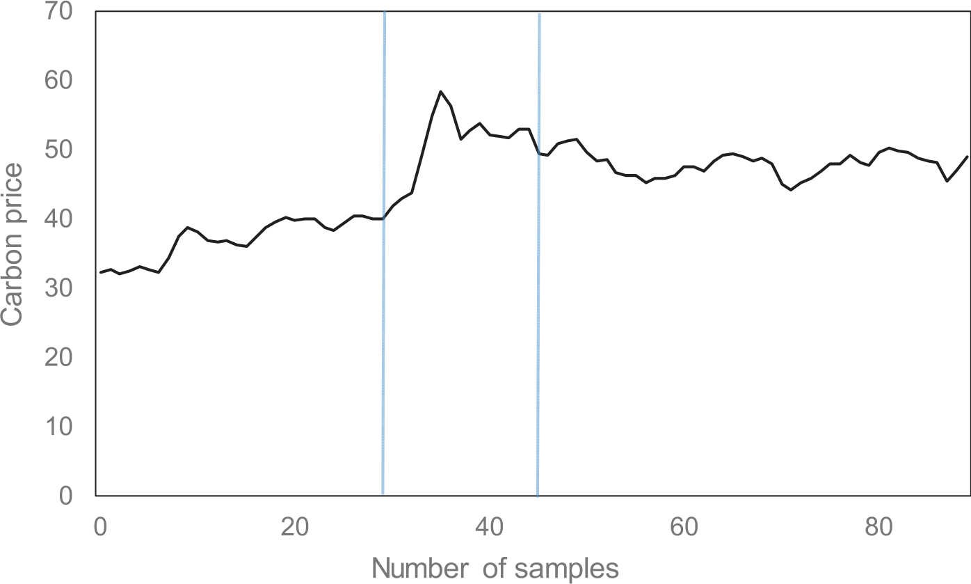
According to the current development trend, if there are no significant changes in the policy and market environment, the carbon price in Hubei will remain in the price range of 45-50 yuan in the coming compliance cycle. Price fluctuations are likely to occur before and after the compliance period, but the amplitude and concentration will be slight. The first reason is that the Hubei carbon market adopts an ex-post adjustment mechanism to allocate carbon allowances and sets different emission control targets according to industry characteristics. Hence, the market’s balance between supply and demand is difficult to break. The second reason is that the market is also very active regularly, and there is rarely a centralized purchase or sale of carbon allowance before and after compliance. However, it is worth noting that the government plans to restart CCER trading, which will transfer some of the spot trading in the market, leading to downside risk in carbon prices.
Comparative Analysis of the Forecasting Effects of Different Forecasting Methods
This paper compares the hybrid model consisting of a random combination of forecasting models such as BP, LSTM, GRU, and BIGRU with decomposition models such as EMD, EEMD, and VMD with the hybrid carbon price forecasting model VMD-BIGRU used in this paper. The standard deviation of white noise for EEMD is set to 0.05, the number of integrations is 100, and the number of nodes in the hidden layer of BP is 5. To enhance comparability, the parameter settings of LSTM and GRU are consistent with BIGRU. The calculation results of the evaluation indicators of different forecasting methods are shown in Table 6.
We compare BP, LSTM, GRU, and other neural networks, which are currently performing well in this field, with BIGRU. The forecasting results of each model are shown in Fig. 11. Regarding forecasting models, the comparison results in Table 6 and Fig. 11 show that the forecasting effect of the BIGRU model is better than that of other neural networks, whether the object is the original series without decomposition or the new series after decomposition by different decomposition models. It can not only accurately grasp the changes in the trend of the forecast samples but also minimize the gap between the forecasting value and the real one, showing that the bidirectional information transfer characteristic of the model has excellent information capture and learning ability for the carbon price series with nonlinearity and high complexity.
Table 6.
Calculation results of evaluation indicators under different forecasting methods.
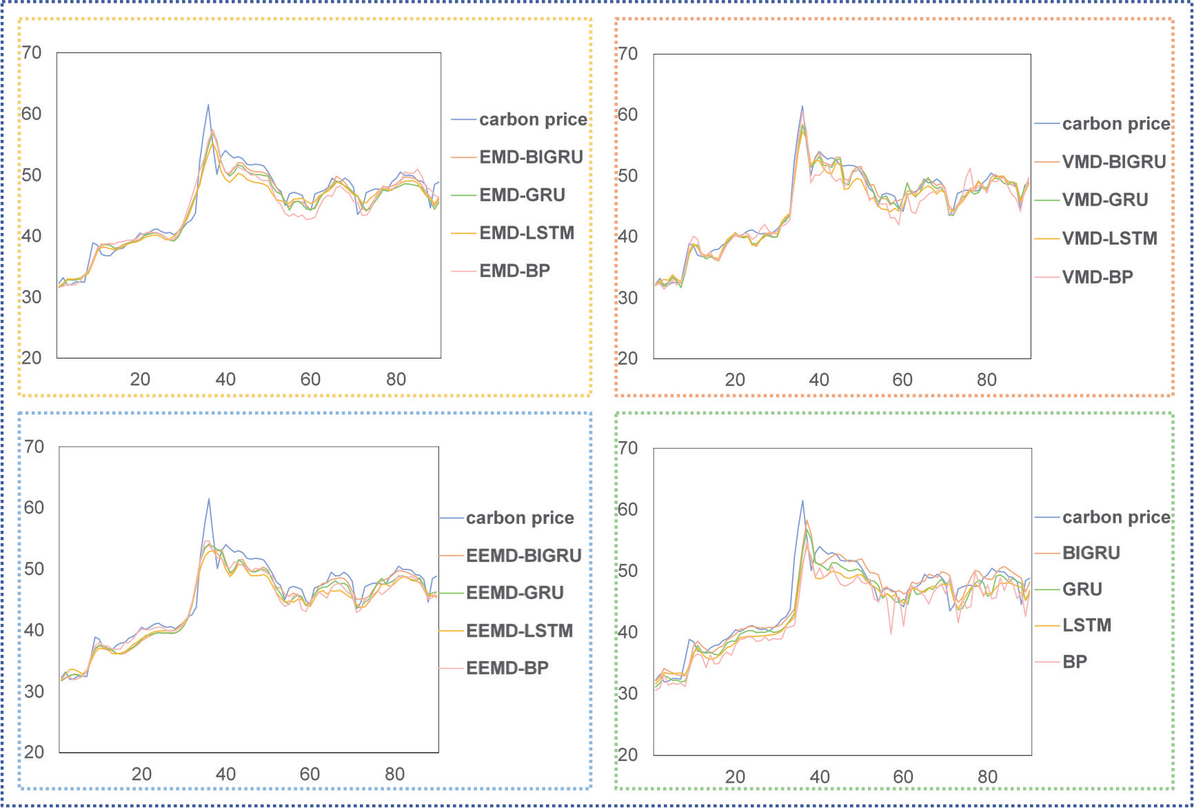
Concerning the hybrid forecasting model, the calculation results of the evaluation indicators of the VMD-BIGRU model are all superior to those of the other comparison models, which undoubtedly demonstrates its suitability for forecasting the carbon price in Hubei. The model’s goodness of fit reaches 96.90%, indicating that the independent variable can explain 96.90% of the changes in the dependent variable in the model through the regression relationship, and the high proportion of explanation reflects the excellent fitting effect of the model. Furthermore, its MAE, MSE, MAPE, and RMSE are 0.8432, 0.1175, 1.84%, and 1.1146, respectively, all the indicators’ lowest values. Dstat is 74.44%, meaning that nearly three-fourths of changes in the trend in the forecasting results are consistent with the actual. It indicates that the model used in this paper is well-equipped to capture the fluctuation trend of the carbon price series.
Although the results of indicator evaluation show that the VMD-BIGRU model has the best forecasting effect, its evaluation results are too similar to the VMD-GRU model, and this weak difference is probably not significant. Therefore, to prove the advantages of the VMD-BIGRU model proposed in this paper more reliably, the DM test is applied to verify the significance of the difference between it and the comparison models. The judgment of this test is based on the difference between the loss series produced during the forecasting process of two comparison models, so the positive and negative statistical values can show the superiority or inferiority of their forecasting effect. At the same time, the p-value represents the significance level of the difference. In Table 7, the DM values are all negative, which means that the forecasting error of the model used in this paper is smaller than all comparison models. The p-values are all less than 0.10, indicating that these differences in accuracy are all significant at a 10% significance level, which more reasonably proves this hybrid model’s high applicability in forecasting the carbon price in Hubei.
Table 7.
DM test results for different models.
Conclusions
This paper combines effective influencing factor screening methods, scientific signal decomposition techniques, and advanced forecasting models to forecast the carbon price in Hubei. Initially, the LASSO algorithm is used to screen out the main influencing factors highly correlated with the carbon price. Secondly, the original carbon price series is decomposed into 8 IMFs and 1 residual series by the VMD model, and the decomposed series is reconstructed into 4 new series named Mode according to their SE values. Afterward, combining the main influencing factors, the new series are forecasted separately by the BIGRU model, and then each forecasting result is summed up to obtain the final forecasting value. Eventually, the forecasting effects of VMD-BIGRU and other models are compared and analyzed regarding evaluation indicators and the significance test of differences. Additionally, the forecasting result is interpreted in light of reality to justify it and further forecast the changes in the carbon price outside the sample.
The main conclusions reached in this paper as a result of the study are as follows:
(1) The BIGRU model can ensure better forecasting accuracy while simplifying the model structure. Regardless of whether the research object is decomposed, its forecasting effect is better than that of other comparison models, and it has a high degree of applicability in forecasting the carbon price in Hubei.
(2) The hybrid carbon price forecasting model constructed by combining the VMD and BIGRU models can show a good combination effect. The evaluation results of its R2, MAE, RMSE, MAPE, MSE, and Dstat are superior to all comparison models set up in this paper, and this advantageous difference passes the DM significance test, further proving its feasibility and excellence.
(3) Carbon prices in Hubei continued to rise in the early and middle phases due to the national carbon market opening, market speculation, and policy inducements. They then gradually dropped and stabilized in the late phase due to the market’s balance between supply and demand and the off-season for compliance. Without significant changes in the policy and market environment, the carbon price in Hubei will remain in the price range of 45-50 yuan in the coming compliance cycle and will experience slight fluctuations before and after the compliance period.
The features and innovations of this paper are mainly in the following two areas: First, the hybrid model VMD-BIGRU is employed in the field of carbon price forecasting, and its applicability in the forecasting task of the Hubei carbon market has been proven, which contributes to the further development and application of the BIGRU model in this field. Second, after the completion of the forecasting, the reasons for trend changes in the carbon price forecasting results are explained in light of the actual market development and changes in the main influencing factors. Then a reasonable forecast is made based on these for future changes in the carbon price outside the sample.
Nonetheless, the research in this paper still needs improvement. Compared with the European carbon market, the domestic carbon market started late, and the development of all aspects still needs to be mature, so there is less sample data to study. Subsequent studies will improve this and focus on the correlation between the policy environment and the carbon market to expand the research scope of the carbon price further and enrich the research content on influencing factors.

