

Introduction
The primary conflict between the social economy’s rapid development and industrial technology’s prompt advancement is the scarcity of water resources, the pollution of the water environment and the damage to water ecology make this contradiction more prominent, therefore, in addition to ensuring ecological security, encouraging the resource usage of wastewater can also help to resolve the imbalance between the supply and demand of water resources. In addition, the supervision and implementation of increasingly strict ecological and environmental management standards and policies make it difficult for the effluent quality of many wastewater treatment plants to meet the discharge standards, of which the total nitrogen (TN) in wastewater effluent is one of the main pollutants. A large amount of excess nitrogen in wastewater discharged into natural water bodies will cause secondary pollution of them, leading to black odor as well as eutrophication, while increasing the difficulty and cost of wastewater treatment and even causing harmful effects on natural species. Hence, the TN concentration should be reduced to the standard level before discharging wastewater into the environment. There are certain limitations while applying the hardware sensors to measure water quality parameters, as time goes on, the accumulated sludge and sediment on the sensors will reduce their accuracy, and will affect theirs service life, increasing maintenance costs, etc. To address the reliance on hardware sensors, soft sensor models provide an effective solution for this purpose. Soft sensor refers to the analysis of data through mathematical theories and thus the construction of models for real-time prediction through indirect measurement methods.
However, the wastewater treatment process is characterized by strong non-stationarity, hysteresis, the complexity of the characteristic variables, and difficulty in modeling [1-4] and traditional prediction model has certain shortcomings on this issue. The conventional gray system prediction model [5] is only appropriate for short- and medium-term prediction of small-scale sample data, which is one of the drawbacks of the general prediction model, and is only suitable for prediction according to exponential growth. In other words, the prediction effect of the gray prediction model is poor when facing the data samples with large variability. Another example is that the regression equation calculation of the regression prediction model [6] is cumbersome, and has high requirements for the distribution of sample data. In recent years, the processing ability of deep neural network prediction models had better performance when facing complex nonlinear functions. However, multilayer neural network prediction models will have gradient disappearance and explosion, which will easily lead to incomplete training.
To address the above problems, an integrated stochastic configuration network (SCN) learning model based on a fractional-order difference algorithm (FDA) to predict effluent TN in wastewater is proposed in this work. To make the input sample data set of the prediction model more stable and adaptable, the FDA is introduced to generate several different training subsets for data sampling, and each small-scale SCN model is generated based on the training of different training subsets, and then each small-scale SCN model is integrated. This sampling method can eliminate the linear convergence of the data and the time dependence of the data, and obtain a smooth series to ensure that the SCN model has better learning ability and can better cope with strong nonlinear data, solve the problem of regression prediction of complex variables, and help improve the prediction accuracy.
Material and Methods
Related Works
Currently, the most widely used water quality parameter prediction model for the wastewater treatment process is neural network modeling. Researchers have conducted extensive studies by using neural network modeling technique for the wastewater quality prediction models [7-10].
Zhang et al. [11] established a BP neural network model for the Mohe River's COD concentration of water quality forecast, which overcomes the limitations and extends the application of the model. Wodecka et al. [12] used a classification model to foresee how the wastewater quality would vary as it entered the wastewater treatment facility, and established a statistical model based on support vector machine and incremental tree methods, which can accurately determine the values of the chosen indicators of wastewater quality. Chopade et al. [13] built a sensor based deep learning method for the wastewater quality prediction model. Four performance metrics are used during the experiment, including precision, recall, accuracy, and F1 score, and the system achieves an accuracy of more than 90%, despite 20% noisy labels. Zhao et al. [14] introduced an extreme learning machine (ELM) based on the lion swarm optimizer to build a soft sensor model and predict the wastewater BOD5 and COD concentrations, and the outcomes demonstrated that the model performs superbly in the prediction of BOD5 and COD. Cong et al. [15] proposed a VSRBFNN model with the variable structure to predict wastewater effluent COD. The VSRBFNN model reduces the complexity of the activated sludge process (ASP) mechanism model, and the proposed soft sensor, while functioning under different conditions, shows good prediction accuracy. Feng et al. [16] used predictive models such as predictive component correlation vector machine, RVM, PCA-RVM, and ICA-RVM to monitor the benchmark simulation model no. 1 (BSM1) platform of wastewater treatment provided by the International Water Association (IWA), and the fault detection accuracy of predictive component correlation vector machine was higher than other models. Du et al. [17] used PSO algorithm to optimize BP neural network to get the model of chromium adsorption in wastewater, and results show that the proposed model’s optimization procedure rapidly conclude with highly accurate predictions for chromium in wastewater.
Although traditional machine learning methods have high accuracy prediction effect, prediction models are easy to implement and understand, and can fit arbitrary continuous nonlinear mapping relations in high-dimensional space, these models usually have only three layers and below of computational units, ignore the correlation between features, and have insufficient generalization ability in the face of more and more complex industrial process data, thus showing certain limitations. Wan et al. [18] utilized the spatial properties of fused convolutional neural networks (CNN), the temporal properties of shared weight long short-term memory (SWLSTM), and the probabilistic dependability of Gaussian process regression (GPR) to the high accuracy interval prediction of paper wastewater treatment systems. The proposed CSWLSTM-GPR model’s predicted values were frequently maintained within the water quality range with improved integrated prediction. Cheng et al. [19] used a deep learning model based on LSTM and the gated recurrent unit (GRU) as a soft sensor to predict the key features of wastewater treatment plants. The proposed model has higher prediction accuracy with faster convergence. Wan et al. [20] proposed to combine the grey correlation algorithm (GRA) and the GRU network into a prediction model to predict wastewater operations, and the GRA-GRU model predicted influent wastewater conditions with better accuracy than GRU, LSTM, CNN, and MLR models. Li et al. [21] and Liang et al. [22] proposed a combined CNN-LSTM deep learning approach based on flow prediction that helps to estimate water availability and flood warnings for watershed management, while in the presence of complex circumstances, the model’s forecast accuracy will decline. Heo et al. [23] proposed a hybrid model based on multimodal and integrated deep learning (ME-DeepL) for predicting wastewater influent water quality, and the experimental results showed that the ME-DeepL model can achieve high accuracy in predicting influent water quality by capturing the information characteristics and temporal trends in influent loads that change. Quang et al. [24] compared six different machine learning algorithms, for predicting total phosphorus (TP) in wastewater effluent, a variety of learning architectures from shallow to deep have been used, including seasonal autoregressive integrated moving average, random forest, support vector machine, gradient tree boosting, adaptive neuro-fuzzy inference system, and LSTM, the experimental results showed that the SARIMAX prediction model is structurally stable and can handle non-smooth large data sets, providing a reliable and accurate method for predicting wastewater effluent quality. Newhart et al. [25] presented a novel hybrid statistical machine learning ammonia prediction model and a statistical stability metric, the proposed methodology can enhance municipal wastewater treatment’s accuracy and precision. Wang et al. [26] employed a novel technique to optimize and forecast TP pollutant removal and turbidity, combining response surface methodology and artificial neural network (RSM-ANN). The methodology can enhance municipal wastewater treatment’s accuracy and precision. They constructed an ANN model with BP algorithm based on RSM data as well as uncontrollable variables, raw TP concentration and raw water turbidity, and the proposed model was able to predict TP in wastewater effluent better.
In deep learning neural networks, due to the complexity of the model structure, the training process of the network usually needs large-scale data for support, and the network convergence speed is slow. Only two adjacent layers are connected since each level uses the output of the previous level as the input for the subsequent level, this kind of structure not only fails to solve the time-series sample set, but even ignores the correlation between the whole and the parts, leading to the inability to make an unbiased estimation of the laws of the data.
Stochastic configuration network (SCN) [27] is a special kind of neural network that uses a random number function for the random assignment of weights compared to gradient-like neural networks. The SCN network achieves asymptotic approximation well while overcoming the problem of network function values falling into local minima and reducing the process of iterative adjustment of network parameters. The structure not only improves the prediction effect of the network, significantly quickens the gradient-based class algorithm’s convergence, and even substantially improves the adaptability of the network model and other problems. However, as the number of nodes in the hidden layer increases, the SCN soft sensor model can be overfitted due to the input data maladjustment and pathological conditions. The fractional-order difference algorithm (FDA) can transform a non-smooth series into a smooth series, and the process of data sampling using the FDA not only ensures the smoothness of the data but also preserves the original information of the data. In view of the above, a soft sensor model for the effluent TN in wastewater based on the FDA-SCN integrated learning network is proposed.
SCN Neural Network
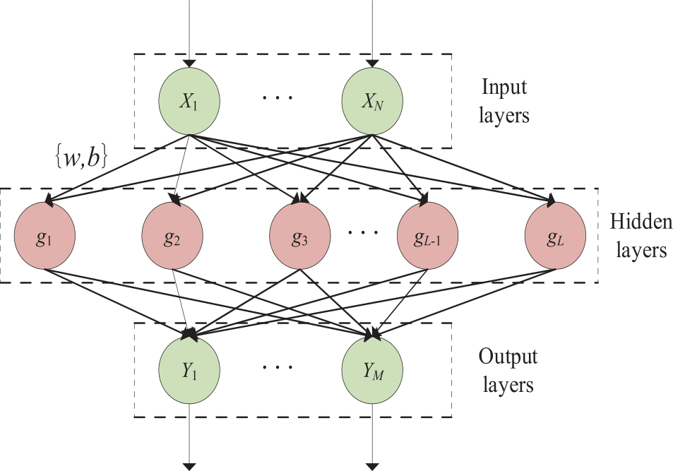
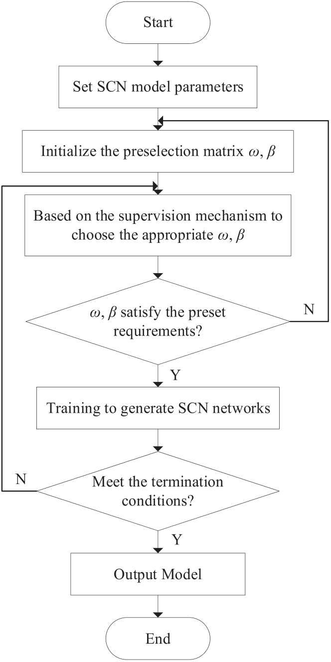
A typical feed-forward neural network topology for an SCN consists of three layers: input layers, output layers, and hidden layers. Its typical network structure is shown in Fig. 1. Assign input weights ω and biases b according to an inequality-constrained least squares algorithm with supervised learning rules, the Sigmoid function is selected as the activation function of the hidden layer of the SCN network, and denotes the number of nodes in the hidden layer by L, the weights and biases of the k-th hidden layer nodes are denoted as ωk and bk, and the hidden layer output is represented as gk:
where, σ(z) is a random basis function, and the calculation of σ(z) is represented as σ(z) = 1/(1 + exp (–z)), here in which
If the hidden layer’s output nodes count in the SCN network are set to M, the output weight of the nodes in the hidden layers is set to β = [β1, β2, ..., βM]L×M, then, for samples, the hidden layer output can be expressed as H = [g1, g2, ..., gL]N×L, and the output Y of the whole SCN network can be expressed as
Fig. 2 displays the SCN algorithm’s basic flowchart.
Fractional-Order Difference Algorithm (FDA)
The difference means that the difference between two adjacent terms in a sequence is a constant, it may be favorable or unfavorable, negative value signifies that the first term in the series is greater than the last term in the sequence, while a positive value indicates the opposite. The difference algorithm is mainly based on the difference between the current item and its predecessor in the sample, because of this, one-dimensional arrays are the primary data types on which the difference technique is used. Integer-order difference may cause the data to lose the information contained in the original sequence and thus remove the memory of the signal, the interpolation of the fractional-order difference algorithm (FDA) uses this property of the Gamma function 0<x<1, FDA is a better solution to the trade-off between data smoothness and preserving data information. The FDA algorithm first loops through the difference values of the input data and stores them in a vector, and then uses the calculated difference values to find the approximate value of the definition domain. It is defined as follows:
Given a time series {X}t = 1, 2, ..., T and order d∈(0,1), then the d order difference equation at time t is:
where, ω0 = 1, ωk = – ωk–1 (d – k + 1)/k. It can be seen that the information of each data point X̃ varies under the influence of the weight ωt, there is a choice to enlarge the data set with a defined information window for this data set.
Soft Sensor Model Based on FDA-SCN Network
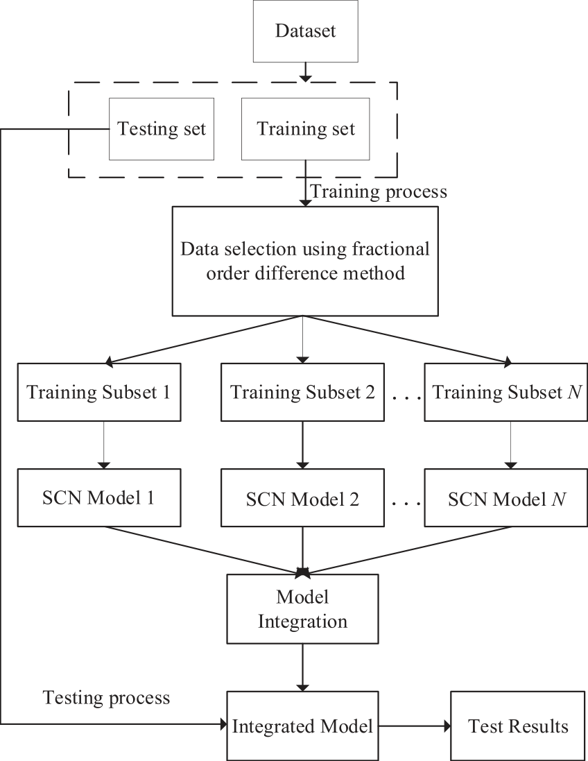
The integrated learning method is used to obtain a more comprehensive strongly supervised learning model by combining multiple weakly supervised learning models, mainly by training multiple sub-models in parallel to accomplish the task. Firstly, the training samples are sampled using adaptive sampling to obtain N subsets. Secondly, independently train N subsets of samples to obtain N sub-models. Finally, an appropriate combination strategy is chosen to integrate the obtained N sub-models. For the integrated network prediction model, the stability of the sub-models is a crucial aspect in determining the prediction model’s accuracy.
The SCN model determines the input weights and bias of hidden nodes by adaptively selecting the range of random parameters, and introduces inequality constraints based on the least squares algorithm to calculate and analyze the output weights selectively. With the increase of the model configuration nodes as well as the number of layers, the SCN can substantially approximate the original function during the training process and maximize the guarantee that the error converges to 0, to have an outgoing TN prediction model with strong generalization ability and a random training method. In this paper, we first use FDA to sample the input samples into multiple sample subsets. The model’s variability is then raised during the training process to improve the SCN network model’s ability to generalize and be stable. The subsets of samples sampled by the FDA are trained independently to generate multiple sub-models, and the sub-models are combined according to a certain combination law. The specific combination strategy is as follows: Input: training data set D, number of sub-learners N,
typical SCN algorithm Output: Integrated learner R(X) Methods:
1) For =1 to N
2) Generate a training subset D of the same size as D by sampling from the training set D using the FDA sampling method Dn
3) N sub-learners are generated by training a typical SCN model based on different training subsets rn(X)
4) End for
5) Integrate N small-scale SCN models, output integrated learner
The flowchart of the proposed soft sensor model of wastewater effluent TN based on the FDA-SCN integrated learning network is shown in Fig. 3.
The FDA is used to sample the input sample set to generate N training subsets, and the different training subsets are used to train in parallel to generate mutually independent SCN models. Meanwhile, to evaluate each SCN model’s ability to forecast TN, the dataset not collected by the FDA is used as a test set to verify the performance of the evaluation sub-models and the final model, and finally, the sub-models are fused into an integrated model.
Results and Discussion
Data Acquisition
Data set I is selected based on the BSM1 simulation platform provided by IWA for data taking in the wastewater treatment process, the simulation platform is made to run under stormy weather conditions for 14 days with 15-minute intervals to collect data, and a total of 1344 sets of data were collected, the auxiliary variables included in BSM1 are shown in Table 1.
Data set II is based on the official website testing of the Ganges River water in India, and one set of data was recorded at one-hour intervals, 10 sets per day, for water quality parameters from July 15, 2022 to September 15, 2022, yielding a total of 600 sets of data with the auxiliary variables included in the water quality of the Ganges River are shown in Table 2.
Data Pre-Processing
To increase the data stability and prediction precision, the original data series are normalized using the extreme values of the variables (maximum and minimum values) to eliminate the influence of units and orders of magnitude on the model. The equation is as follows:
where, X' stands for the value of a particular piece of data, min is the column’s minimum value, and max is the column’s maximum value, and each of these terms refers to the value of the data in question.
Feature Extraction
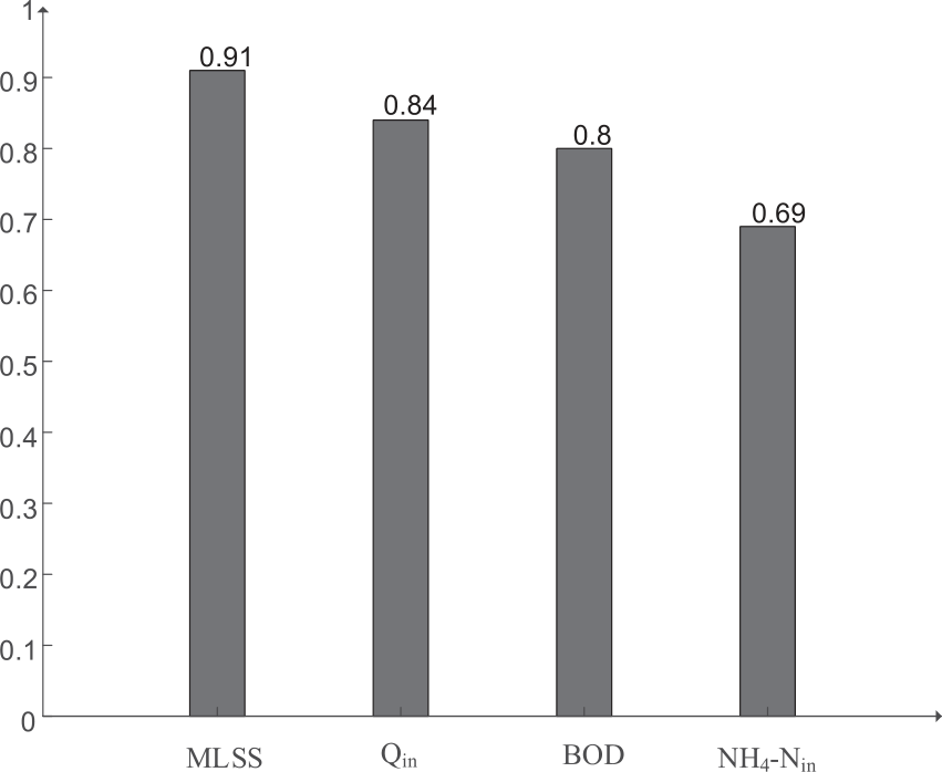
The gray correlation method is based on the linear interpolation method to transform the discrete observations of the characteristic variables into continuous lines between the intervals, and observe the similarity between the curves of the intervals, to determine the degree of correlation between the characteristic variables, which applies to data sets of any regularity and size. The gray correlation method calculates the fit between the comparison series and the reference series through the quantitative analysis of the dynamic process of the features, and ranks the importance of the sample series according to the magnitude of the correlation between the series, depending on the ranking, chooses the feature variables with the highest correlation and relevance as the model’s input features.
Table 1.
BMS1 characteristic variables.
Table 2.
Ganges water quality characteristics variables.
The gray correlation model is run multiple times to do an importance analysis of the data, and the correlation values of the results of multiple runs are used as the basis for importance ranking.
Fig. 4 displays the distribution of the sample features’ relevance based on the BSM1 simulation data’s gray correlation model. Seven parameters such as Qin, BOD, COD, MLSS, SNH3, SND, and XND are selected as the input features of the model.
Fig. 5 shows the important distribution of the sample characteristics of the Ganges River water quality parameters output under the gray correlation model. Five characteristics, such as influent flow TSS, Temperature, BOD, Nitrate, and COD, which are highly correlated with the effluent TN, are selected as the inputs to the model. Where, (1) TSS is the total amount of non-dissolved suspended solids floating in water. Some nitrogen compounds may bind to suspended floating particles, thus affecting their migration and availability.
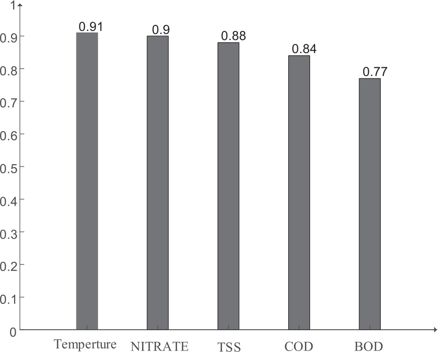
(2) Temperature affects the biochemical processes and nitrogen transformation processes in the water column. Higher temperatures may lead to an increase in the rate of biotransformation of nitrogen compounds, thus affecting the total nitrogen concentration. (3) BOD is the amount of oxygen required for organic pollutants to be degraded by microorganisms in water. Organic pollutants may contain nitrogen compounds, and their biodegradation processes may release nitrogen compounds, which in turn affect the total nitrogen concentration. (4) Nitrate is an important nitrogen compound that is the end product of ammonia oxidation and nitrification processes. Increases in nitrate concentrations may correlate with changes in total nitrogen concentrations, especially in water bodies contaminated with nitrate or eutrophic.
(5) COD is the total amount of oxidizable substances consumed in water, which includes both organic and inorganic substances. an increase in COD may imply an enrichment of organic substances, which may interact with nitrogen compounds and thus affect the total nitrogen concentration.
Considering that many different factors may affect the total nitrogen concentration in the effluent, for example, the process of nitrogen transformation may be affected by aerobic/aerobic conditions, and the presence of different microbial communities and changes in environmental factors (such as oxygen concentration, pH, etc.) may also affect the transformation of nitrogen compounds and total nitrogen concentration. Therefore, the gray correlation algorithm is employed in this paper to make importance analysis of the characteristic variables affecting TN concentration, and selects five specials, including TSS, Temperature, BOD, Nitrate and COD, with correlation degree greater than 0.75 as the input of the model to simplify the complexity of the input characteristic variables [28].
Model Training
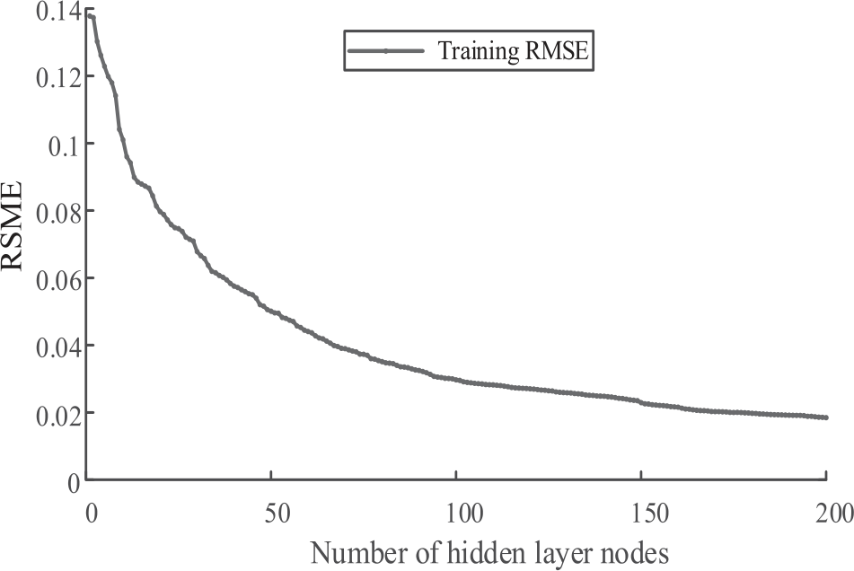
The relationship between the number of hidden layer nodes and the training error for each sub-model SCN is shown in Fig. 6.
Depending on the size of the input data set and the FDA-SCN model’s guiding principles, the training termination condition is set as: maximum number of nodes in the hidden layer Lmax = 200, allowable error ε = 0.01. The weight parameter is set to FDA-SCN model the maximum number of search iterations Tmax = 150, the range of random weights is set to {0.5, 1, 10, ..., 150, 200, 250}, inequality constraint factor is r = {0.9. 0.99, 0.999, 0.9999, 0.99999, 0.999999}.
Analysis of Results
In this study, the FDA-SCN model’s effluent TN prediction effect is evaluated using the correlation coefficient (R2), mean absolute percent error (MAPE), and root mean square error (RMSE), which are described by Equations (6), (7), and (8). The model’s number of samples is set to n, yl is the simulated predicted value of FDA-SCN prediction model, and yi is the actual value of effluent TN.
Soft Sensor of TN Concentration Based on BMS1 Simulation Platform Data
Table 3 shows the RMSEs of FDA-SCN model and SCN model at different hidden layer nodes with the same hyperparameters set, and the prediction error values of FDA-SCN model at different nodes are much lower than those of SCN model, and Fig. 7 depicts the relationship between the actual effluent TN concentration and the projected values from the FDA-SCN and SCN models. It can be seen that the predicted value of FDA-SCN model has a higher fit with the actual value of effluent TN, which in turn indicates that the FDA-SCN model has a more accurate prediction effect, and the FDA-SCN prediction model designed in this paper is better than the single SCN model.
Table 4 demonstrates the superiority of the FDA-SCN model for MAPE, RMSE, and R2 performance compared to deep learning neural networks CNN-LSTM, LSTM, and shallow neural networks BP, Elman, ELM, FDA-ELM, and other prediction models. The RMSE, MAPE and R2 are 0.01866, 0.016381 and 0.96387, respectively, demonstrating how the FDA-SCN model developed in this paper might enhance the predictability of wastewater effluent TN.
Table 3.
RMSEs at different nodes.
| Models | The test performance corresponding to different nodes (RMSE) | |||
|---|---|---|---|---|
| 50 | 100 | 150 | 200 | |
| SCN | 0.094885 | 0.061482 | 0.045729 | 0.038147 |
| FDA-SCN | 0.048312 | 0.031345 | 0.023251 | 0.018666 |
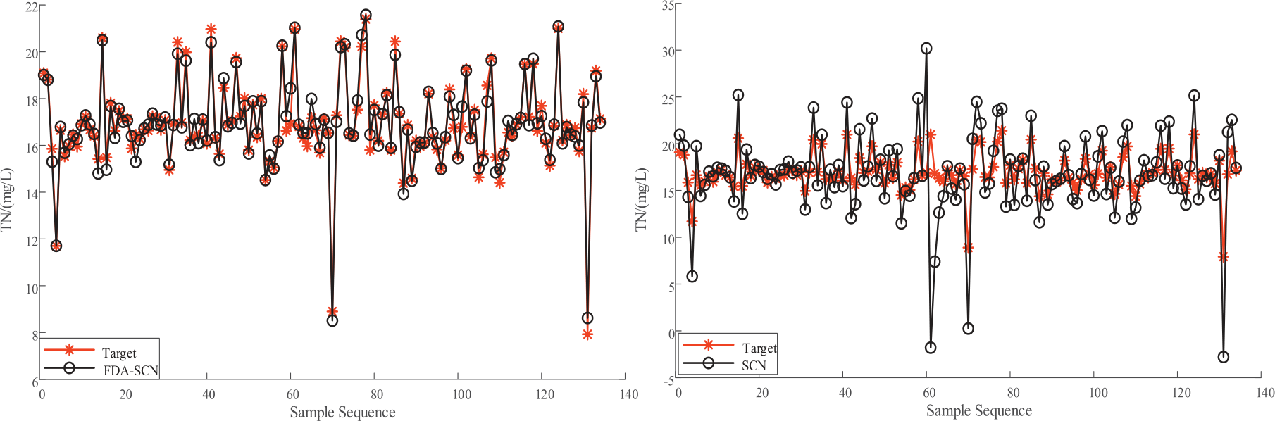
Table 4.
Comparison of different model predictors.
| Models | RMSE | MAPE | R2 |
|---|---|---|---|
| BP | 1.1964 | 0.05853 | 0.63372 |
| Elman | 1.8732 | 0.075137 | 0.06605 |
| LSTM | 1.7624 | 0.074875 | 0.20743 |
| CNN-LSTM | 0.13217 | 0.08034 | 0.34300 |
| ELM | 1.4461 | 0.68166 | 0.79154 |
| FDA-ELM | 0.87614 | 0.040522 | 0.79154 |
| FDA-SCN | 0.01866 | 0.016381 | 0.96387 |
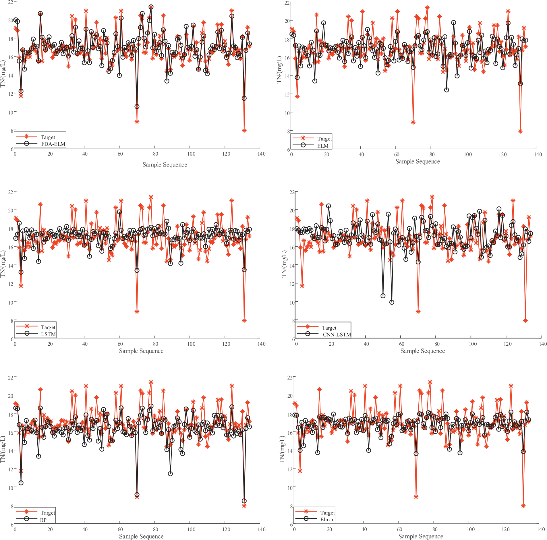
Fig. 8 respectively demonstrates that when compared to shallow and deep neural networks, the relationship curve between the projected value and the actual value is simulated by each model. The results indicate that, in comparison to other neural network prediction models, the TN prediction value of the FDA-SCN model has a better agreement with the actual value, additionally, the error fluctuation range is consistently smaller than that of other models, which verifies the accuracy of the prediction model proposed in this paper.
Soft Sensor of TN Concentration Based on Water Quality Data of Ganges River
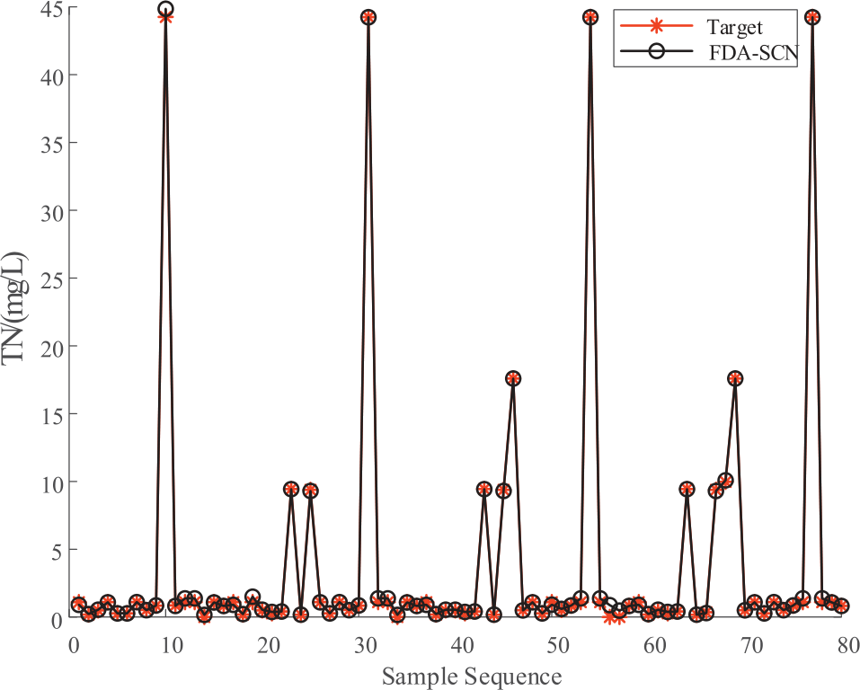
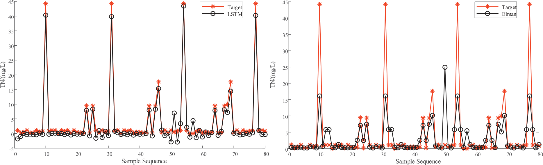
To further verify the validity and robustness of the designed model, the FDA-SCN prediction model is applied to the real-time collected water quality data of the Ganges River in India as the input eigenvalue variable, for the purpose of real-time prediction of the effluent TN concentration. The training set and the test set were randomly assigned. Fig. 9 displays the results of the FDA-SCN model’s comparison of the expected and actual values of TN concentration. It is clear from the figure that the fit between the predicted and real values of wastewater effluent TN is significant, indicating that the FDA-SCN model has a stable structure and good prediction effect. In order to confirm that the FDA-SCN prediction model is superior, Elman and LSTM models were selected as the comparison network to predict the effluent TN under the condition of the same input samples. The relationship curves between each model are shown in Fig. 10, which shows that the error fluctuation range between the FDA-SCN model’s predicted value and the actual value of effluent TN is always smaller than that of other prediction models, and the proposed model’s prediction accuracy is consistently higher than that of other models.
The comparative results of FDA-SCN model in terms of MAPE, RMSE and R2 performance are shown in Table 5. The FDA-SCN model has the highest prediction accuracy for the effluent TN concentration under the influence of multiple parameters, according to the comparison of the indicators. This finding suggests that the method developed in this paper has a more stable network structure, stronger generalization ability, and more accurate prediction effect, and can be successfully applied to the soft sensor of key water quality parameters for the real world using.
Although the soft sensors based on FDA-SCN network is proposed for monitoring the water quality in wastewater treatment process, it can also be used to monitor the water quality of natural water bodies in real time. The data collected by the physical sensor from the water body (e.g., temperature, nutrient concentrations such as nitrogen and phosphorus) would be feed into the model for real time analysis to predict target concentration. FDA-SCN model can predict water quality changes, identify the impact of plant activity on water quality and predict future water quality trends. For water quality monitoring in natural water bodies, soft sensors can provide real-time data and warnings that can help identify water quality changes early.
Conclusions
To solve the problems of complex auxiliary variables of effluent TN concentration in wastewater treatment process, poor prediction accuracy, unstable prediction model structure, difficult online real-time measurement and long prediction time, an integrated FDA-SCN soft sensor model is proposed in this work. The conclusions are as follows:
(1) The study of FDA sampling method can solve the problems that when the input sample data size is large, the deep neural network soft sensor model is easy to cause the loss of critical interest and long training time, and the shallow network soft sensor model structure is unstable and the training error fluctuates widely. The FDA sampling method can ensure the smoothness of the data while preserving the memorability of the original data, which speeds up the convergence of the algorithm.
(2) The FDA-SCN integrated learning model proposed in this study overcomes the randomness of the gradient-like neural network in the process of model convergence that makes the model parameters and structure occur, prevents the network’s propensity to enter local minima, avoids the network’s propensity to enter local minima, and significantly increases the soft measurement model’s generalization and accuracy.