

Introduction
Floods are the most destructive natural catastrophes, leading to losses in human lives, infrastructure, crop yields, and industrial production. It can also seriously affect the environment and the social lives of people in terms of electrical damages and risks, contaminated water, sanitary hazards, problems in drainage, and destruction of roads and other communication networks. A flood is a situation when water overflows from a watercourse (river, lake, or stream channel) and comes to the land, which is usually dry [1-4]. The main reasons behind floods are heavy rains, melting glaciers, breakage in reservoirs used for water storage, and a lack of river channels to effectively convey the excess water [5-7]. Floods are natural phenomena occurring at irregular intervals of time. The flood frequency analysis is used with the objective of predicting the recurrence of flood levels for different return periods. Such prediction of floods is important for certain planning at the government and country level, like the construction of water reservoirs, spillways, bridges, canals, and culverts. It is also important to plan disaster management activities (including protection of human lives, assets, and food security) for any possible hazard in the future. Flood frequency can be carried out with different approaches, like the California method, the Hazen method, and Gumbel’s method [1]. The flood analysis can be carried out at the country, regional, or site level. At-site flood frequency analysis is the most appropriate, effective, and simple way to predict flood recurrence at a particular gauging station [5, 6, 8-11].
The choice of the probability model blended with an appropriate estimation strategy plays a vital role in the modeling of flood data. Each distribution has its own advantages and disadvantages in describing flood data. There can be different probability distributions with different parameter estimation methods suitable for modeling maximum water flow data from different gauging sites. In the literature concerning at-site flood frequency analysis, different probability distributions like Generalized Extreme Value (GEV), GEV type-1, GEV type-2, normal, generalized normal, two-parameter lognormal, three-parameter lognormal, two-parameter gamma, three-parameter gamma, Pearson type-III, Gumbel, reverse Gumbel, exponential, generalized logistic, four-parameter Wakeby, five-parameter Wakeby, and generalized Pareto have been applied for flood frequency analysis of different rivers in different countries [1, 5, 6, 12-18]. A brief review can be seen in some studies [19-21].
Following the findings of many studies for different rivers in the world, we have used Generalized Logistic (GLO), Generalized Extreme Value (GEV), Gumbel (GUM), Generalized Pareto (GPD), and Reverse Gumbel (REV.GUM) distributions for at-site modeling of annual maximum flood data at 5 sites of the Chenab River. Some of these probability models were also used by Ahmad et al. [22] for at-site analysis of many gauging sites, including those of the Chenab River, but with relatively smaller sequences of peak flow data.
Several estimation methods are available for parameter estimation of probability models used for flood frequency analysis. In the present study, we have applied L-Moments (LM), Maximum Likelihood (ML), Least Squares (LS), Weighted Least Squares (WLS), and Relative Least Squares (RLS) methods for estimating the parameters of considered probability distributions.
The performance of each probability distribution estimated with a particular estimation method is assessed based on different goodness-of-fit tests and accuracy measures.
The present study is focused on at-site flood frequency analysis of the Chenab River, with the prime objective of identifying the most suitable probability distribution with a parameter estimation method for modeling the annual maximum discharge data of different gauging sites of the Chenab River. After identifying the most appropriate probability distribution and estimation method for each gauging station, the maximum annual peak flow for different return periods with a specific non-exceedance probability has been estimated.
The rest of the article is structured as follows: Section 2 provides a brief description of the Chenab River and the data used in the current work. Section 3 describes the candidate probability models and parameter estimation methods. Section 4 presents and discusses the results obtained by applying different probability distributions with estimation methods at different gauging sites. Finally, conclusions drawn from the study are presented in Section 5.
Data and Gauging Sites
The Chenab River is one of the major rivers in Punjab Province, Pakistan. The river flows from northeast to southeast directions and enters Pakistan’s Punjab province from Indian Punjab. It measures 960 Km with an approximate enactment area of 29000 km2. Its average annual flow is 12.38 MAF [23]. A map of the Chenab River showing the considered gauging sites is reproduced from Magsi and Atif [24] in Fig. 1. The data have been collected from the Hydrological Directorate of Discharge and Flood Zone, Lahore. The range of the data is different for different gauging sites, varying from 48 to 90 years. The longitude, latitude, elevation, and length of the data series for each gauging site are given in Table 1. The maximum annual flow at each gauging site is graphically represented in the form of time plots in Fig. 2.
Materials and Methods
The choice of a probability distribution and estimation method is vital in any at-site flood frequency analysis. In the following sub-section, a brief introduction of candidate probability distributions and estimation methods used in the current study is provided.
Candidate Probability Distributions
The choice of a suitable probability distribution is vital in any at-site flood frequency analysis. Many probability distributions have been used for flood frequency analysis in different countries. For the analysis of five gauging sites of the Chenab River, we have used Generalized Logistic (GLO), Generalized Extreme Value (GEV), Gumbel (GUM), Generalized Pareto (GPD), and reverse Gumbel (REV.GUM) probability distributions. These distributions are applied and found plausible for at-site flood frequency analysis of different rivers and also for other environmental variables [14, 25-30].
L-Moments (LM) Method
Introduced by Hosking [31, 32], the L-moments are linear combinations of probability-weighted moments (PWM). Being the direct measure of the scale and shape of the data, L-moments are more suitable and convenient than probability-weighted moments. However, it is common practice to compute L-moments using PWM [5, 33, 34]. Theoretically, the rth PWM βr, for a probability distribution with a quantile function φ(F), is defined as:
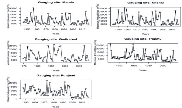
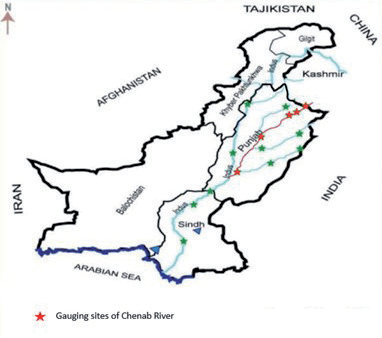
Table 1.
Brief of gauging sites.
For sample data, the first four PWMs are computed as:
Consequently, the first four L-moments are computed by the following relationships,
Hosking [32] defined the coefficients of variation (τ2), skewness (τ3) and kurtosis (τ4) in terms of ratios of the L-moments as:
Just like the method of moments, parameter estimation through the L-moments approach is done by solving a system of simultaneous equations obtained by comparing theoretical and corresponding sample L-moments. The LM method has gained much attention recently due to its computational simplicity [5, 6, 12, 35].
Maximum Likelihood (ML) Method
Maximum Likelihood (ML) is a widely applied estimation method. It gives those values as parameter estimates for which the likelihood, or log-likelihood, attains its maximum. Let us have a random sample of n observations x1, x2,... xn from probability density function f(xi|θ) where θ is the vector of unknown parameters. Let the likelihood and log-likelihood of n independent observations are
Least Squares Method
The Least Squares (LS) method is commonly used for parameter estimation in probability models [37- 39]. It is based on minimizing the following objective function:
where F(xi) is the theoretical CDF of the corresponding probability distribution while i/(n+1) is the sample or observed CDF of the data. This can be done by solving the system of equations obtained by taking derivatives of the above function with respect to unknown parameters. The details can be seen in Ali [37]. For complex functions, the parameter estimates can be obtained by a suitable optimization algorithm.
Weighted Least Squares Method
As proposed by Bergman [40], Weighted Least Squares (WLS) is a variant of the LS method. Instead of identical weights for all observations, WLS uses different weights for different observations. Specifically, in the WLS method, parameter estimates are obtained by minimizing the following function:
Following different studies [41-44], we have used weight function as:
Relative Least Squares Method
Proposed by Pablo and Bruce [45], Relative Least Squares (RLS) is another variant of the LS method. Instead of squared errors (as in the LS method), the RLS method is based on minimizing the squared relative errors. Recently, RLS is reported to be a better performer, in the case of some two-parameter probability distributions [46-48]. Parameter estimates through the RLS method can be obtained by minimizing the following function:
Performance Indicators
To suggest the most suitable probability model for a particular gauging site, the performance of candidate models with an estimation method is assessed. The performance comparison is carried out using some common measures of accuracy and goodness-of-fit (GOF) tests. The test statistics of the GOF tests used in the current study are defined as:
Kolmogorov-Smirnov (KS) test,
Anderson-Darling (AD) test,
Cramér–von Mises (CVM),
Similarly, accuracy measures like Root Mean Square Error (RMSE), Root Mean Square Percentage Error (RMSPE), Mean Absolute Error (MAE), and Mean Absolute Percentage Error (MAPE) are defined as:
In the above GOF tests and accuracy measures, Fn(xi) represents the observed or empirical CDF and F̂ (xi) is the expected CDF of the distribution with particular parameter estimates. Similarly, xi represents the observed value, while x̂i is the estimated value using particular parameter estimates.
Estimation of Quantiles
The estimation of maximum peak flow for a particular return period (T) xT is a major objective of any flood frequency analysis. The recurrence interval T is expressed in terms of years, in which the maximum peak flow xT is expected to return. A specific flood level xT (T being the return period) may be exceeded once in T years. Therefore,
The quantile xT can be estimated by putting F in the quantile function of the corresponding probability distribution. If the quantile function of a probability distribution cannot be expressed in closed form, then the numerical relationships between xT and F can be used to evaluate xT for a given value of F. The quantile estimate for a return period of T years is just computed by inserting value F = (1–1/T) in the quantile function. The standard errors of these flood levels for different return years were estimated, and hence 95% confidence intervals were constructed using the parametric bootstrapping approach [5, 6, 49].
Results and Discussion
The descriptive statistics of maximum annual discharge data from different gauging stations are given in Table 2. From these summary measures, it can be seen that, on average, Khanki gauging station has the maximum annual peak flow, and this particular site also has a higher variation in the maximum yearly flow. Generally, we see that variability in annual maximum peak flow is not too different for different gauging stations, which is evident from values of the coefficient of variation ranging from 66.45% to 70.25%. Randomness, independence, stationarity, and skewness are the core assumptions for the data to be used in flood frequency analysis through probability models [6, 49, 50]. In the current article, we used the Wald-Wolfowitz (WW) test for testing randomness and the correlation coefficient at lag-1 for assessing independence, while the assumption of stationarity was tested using the Augmented Dickey-Fuller (ADF) test. The results of testing these assumptions are given in Table 3. From the p-values of the ADF and WW tests in Table 3, it is clear that assumptions of stationarity and randomness seem reasonable for all gauging sites considered in the study. Moreover, values of serial correlation at lag-1 do indicate that there is no serious/severe violation of the independence assumption. Similarly, values of the coefficient of skewness indicate that the data series for all gauging stations is positively skewed.
The validity of these assumptions justified the application of considered probability distributions for modeling of the annual maximum peak flow data for all gauging sites.
The parameter estimates through LM, ML, LS, WLS, and RLS methods for all of the candidate probability distributions are given in Tables 4-8 for gauging sites at Marala, Khanki, Trimmu, Qadirabad, and Punjnad, respectively. The parameter estimates are accompanied by standard errors (in parenthesis) computed using the parametric bootstrapping approach [5, 6, 49]. The comparative performance of different probability distributions with estimation methods is also given in Tables 4-8. The performance is assessed in terms of the total number of ranks based on three GOF tests and four accuracy measures. For each gauging site, the blend of probability model and estimation method is compared by ranking based on GOF tests and accuracy measures. The highest rank is given to the highest p-value (in the case of GOF tests) and the lowest value (in the case of accuracy measures). The total rank score computed by adding all ranks is given for different combinations of probability distribution and estimation methods. The probability distribution with the maximum total rank is considered to be the most suitable for the particular gauging site.
Table 2.
Descriptive statistics of annual maximum discharge (m3/s) of the Chenab River.
Table 3.
Results of testing assumptions of data from different gauging sites.
From these tables, it turns out that Generalized Pareto (GP) distribution with LS estimation is more suitable for Marala and Khanki gauging stations, as this blend of probability distribution and estimation method got the highest rank based on seven different performance indicators. For gauging sites at Qadirabad and Punjnad, GP distribution with the WLS method provides more accurate and precise results. Generalized extreme value distribution with ML estimation is best suited for the gauging site at Trimmu. It is noted that the GP distribution with LM and WLS estimations performs equally well for Punjnad.
Table 4.
Parameter estimates and performance comparison (Gauging site: Marala).
Table 5.
Parameter estimates and performance comparison (Gauging site: Khanki).
Table 6.
Parameter estimates and performance comparison (Gauging site: Qadirabad).
Table 7.
Parameter estimates and performance comparison (Gauging site: Trimmu).
Table 8.
Parameter estimates and performance comparison (Gauging site: Punjnad).
Table 9.
Estimated flood quantiles for different return years with 95% confidence intervals.
From these results, there is no single probability distribution that fits best for all gauging sites. This finding is in line with the other studies focused on at-site flood frequency analysis [5, 6, 22]. From the results, it is also clear that GP distribution with LS and WLS estimation is a suitable model for most of the sites. As there were varying sample sizes for different sites, it means that sample size does not have an impact on the performance of GP distribution. It is interesting to note that for all gauging sites, the most suitable probability model with one estimation method is also among the top performers with other estimation methods.
Once the best-fit probability distribution is chosen for any particular site, the next objective of the flood frequency analysis is to compute quantiles for different return periods. Such quantiles for different return periods are computed using quantile functions and parameter estimates of the most appropriate blend of probability distribution and method of estimation. For each gauging site, the quantile estimate xT with non-exceedance probability F for return periods 5, 10, 25, 50, 100, 200, 500, and 1000 years is given in Table 9. Uncertainties are always associated with the estimated flood quantiles computed for different return periods. To give an idea of these uncertainties, Table 9 also contains the 95% confidence intervals for estimated flood quantiles using parametric bootstrapping standard errors. For all gauging stations, the values of standard errors indicate that there is more uncertainty in flood estimates for longer return periods as compared to estimates of relatively short return periods.
Conclusions
The modeling of maximum annual discharge at different gauging sites of the Chenab River is done through different probability models blended with different estimation methods. To recommend the best-suited pair of probability models and methods of estimation for each gauging site, we compared the performance of GLO, GEV, GUM, GP, and REV. GUM distributions were estimated with the LM, ML, LS, WLS, and RLS methods. The comparison is based on the total rank of 7 different measures of fit. For each gauging site, the probability distribution with the highest total rank score is considered most appropriate.
Different probability distributions emerge as most suitable for flood frequency analysis at different sites. Generalized Pareto with LS estimation is the most suitable distribution for Marala and Khanki gauging sites. For gauging sites at Qadirabad and Punjnad, GP distribution with the WLS method is found to be the most suitable combination, while GEV distribution with the ML method performs better than all other distributions for the Trimmu gauging station. It can be concluded that GPD with LS and WLS estimation is the most suitable combination for most of the gauging stations (in fact, for all sites except for the gauging site at Trimmu). The results are well in line with many studies focused on at-site flood frequency analysis of rivers in different countries. The emergence of different best-suited probability distributions for different gauging sites has been reported in many other studies [5, 6, 9-11, 22]. Similarly, our finding about the larger uncertainty associated with longer return periods is common and reported in different studies [5, 6].
These results can be used to study and forecast flood levels, the management of water reservoirs, and the planning of hydraulic structures at the Chenab River (and related catchment areas). The most suitable distributions recommended for different gauging sites can be useful candidate distributions for regional analysis of the Chenab River or at-site analysis of other rivers in near geographical locations.
Limitations
Like every research project, the present study also has certain limitations, and work can be done in the future to overcome them. For instance, some other probability distributions, particularly four or five parameter distributions, can be applied. Similarly, different other estimation methods can be used for parameter estimation, like the method of maximum product spacing, Bayesian estimation, etc. Moreover, the analysis can be improved by incorporating a multivariate structure by taking temperature, rainfall, humidity, and other environmental factors into account.