

Introduction
Floods are the most destructive natural disasters that cause losses of lives, land, infrastructure, and agricultural and industrial production, and hence are considered to be one of the biggest threats to the socio-economic fabric in affected areas. It can also create adverse social and environmental problems like disturbance in electricity supply and associated risks, contamination in drinking water, sanitary and drainage hazards, and destruction in communication networks [1-4]. A flood is actually a phenomenon representing the overflow of surplus water from a river, lake, or any other water channel to land outside the usual path of that river or lake. Floods are primarily caused by melting glaciers, extreme rains, leakage or breakage of dams or other water storage infrastructures, or the incapacity of rivers or water streams to pass the sudden additional amount of water [5-10]. Floods are natural disasters that recur over time with irregular intervals. It is a continuous hazardous phenomenon that has affected humans across different time periods. Flood frequency analysis (FFA) is an important way of predicting the time of occurrence of certain levels of floods in the future, which is necessary for planning and designing water reservoirs, disaster management, and other related activities [3, 11-14]. In the literature, different approaches (like California, Gumbel, and Hazen) are recommended for analyzing the frequency of floods [5, 15]. For modeling the stream flow or flood frequency, there are different approaches, like at-site, regional (considering different gauging stations as a homogeneous region), or country-level (one model for all sites in the country), that can be applied. The at-site FFA is the simplest and most direct method for predicting flood magnitude and its recurrence time period with a certain probability for any particular station of any river [2, 9, 10, 16, 17]. A regional approach for FFA is a useful option if data from individual gauging stations is not available for long time periods [18, 19].
For at-site FFA, the data series is assumed to follow a parent probability distribution, and then the parameter estimates of that distribution are used to predict certain flood magnitudes in the future. The optimal choice of distribution and estimation strategy is pivotal in achieving more accurate flood predictions, but there is no general agreement in the literature about any single probability distribution or any particular estimation method [3, 11, 20]. Each probability model has its own advantages and disadvantages in modeling any particular station’s flood data, and different models can be suitable for different stations. For FFA of many rivers in different countries, varying probability distributions have been recommended, including (but not limited to) normal, exponential, generalized normal, two-parameter lognormal, three-parameter lognormal, four-parameter Wakeby, five-parameter Wakeby, two-parameter gamma, three-parameter gamma, generalized logistic, Pearson type-III, generalized extreme value, Gumbel, and generalized Pareto [5, 9, 10, 21-23]. Some very informative and comprehensive reviews on the collection of probability distributions used for FFA in different countries are available in the literature [2, 24-30].
For at-site modeling of annual peak discharge at two gauging stations of the Sutlej River, we have applied Generalized Logistic (GLO), Gumbel (GUM), Reverse Gumbel (REV-GUM), Generalized Pareto (GP), and Generalized Extreme Value (GEV) as candidate probability distributions. These distributions have been applied and recommended for FFA in different studies focusing on different rivers in different countries around the globe [5, 10, 21, 31-35].
Different approaches for the parameter estimation of probability distributions are available in the literature. However, as far as the distributions used in FFA are concerned, methods of L-moments and maximum likelihood are applied in most cases. The maximum likelihood method is one of the widely applied estimation methods, while the L-moments method recently attained widespread attention, particularly in hydrological studies, due to its computational simplicity [3, 9, 10, 21, 36]. However, the least squares method and its variants also provided efficient estimation and were recommended in different cases [37]. Therefore, in the current work, we employed various estimation methods for estimating the parameters of candidate probability models. These methods are L-Moments (LM), Maximum Likelihood (ML), Least Squares (LS), Weighted Least Squares (WLS), and Relative Least Squares (RLS).
The article aims to find the optimal mixture of distribution and estimation method for modeling yearly extreme flow data taken from different gauging sites located along the Sutlej River separately. The performance of each amalgamation (mixture of distribution and estimation method) is assessed based on different performance metrics. For each gauging site, we have evaluated 25 models (5 probability distributions, each estimated with 5 different estimation methods).
Once the best-fit model (blend of distribution and estimation method) for a particular site is identified, it is used to estimate annual extreme discharges for many return years (like 5, 10, 25, 50, 100, 200, 500, and 1000) with a certain non-exceedance probability.
The remaining part of the article is organized as follows: Section 2 gives an overview of the locations of the Sutlej River and data utilized in this study; Section 3 outlines the candidate probability distributions and methods for the parameter estimation applied in this work; Section 4 provides the results and comparative analysis of applying various mixtures of probability distributions and estimation techniques; and Section 5 summarizes the significant findings and conclusions that can be inferred from the current analysis.
Study Locations and Data
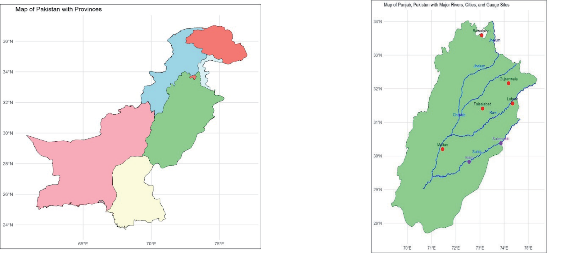
The Sutlej River is a key waterway that plays a vital role in agriculture and other related activities in the southern part of Pakistan’s Punjab province. The river flows northeast to southeast, entering Pakistan from the Indian Punjab. In Pakistan, it covers a distance of around 350 km before merging into the Chenab River at Panjnad. Fig. 1 represents a map of the Sutlej River with gauging sites in Pakistan’s Punjab province.
The data for this analysis was obtained from the office of the hydrological directorate located in Lahore, which is responsible for measuring water flows at different barrages in the Punjab province. The data spans 50 to 52 years for two gauging stations located in Pakistani territory. Table 1 provides important characteristics (such as time period of data series, elevation from sea level, and geographic coordinates) of gauging sites considered in the current work. Fig. 2 provides time series plots of the maximum annual flow at each gauging station for a visual representation.
Materials and Methods
An optimal combination of probability distribution and estimation method is crucial for conducting any FFA [2, 38, 39]. This is because the right choice of this blend is vital for efficient modeling and hence accurate estimation of flood levels for different future time periods. We utilized GLO, GUM, REV-GUM, GP, and GEV distributions in our at-site FFA of gauging sites along the Sutlej River. We applied LM, ML, LS, WLS, and RLS methods to estimate the parameters of these distributions. The following subsections briefly discuss the probability distributions and parameter estimation methods being compared.
Candidate Probability Distributions
Several probability distributions, each with its own merits and demerits, have been found useful for FFA across different countries. Table 2 gives the probability density functions f(x), cumulative distribution function (CDF) F(x), and quantile functions φ(F) of the distributions applied in the current work. These distributions have been applied and found suitable for FFA for different river sites in many studies.
Here, location, scale, and shape parameters are denoted by µ, α, and β, respectively.
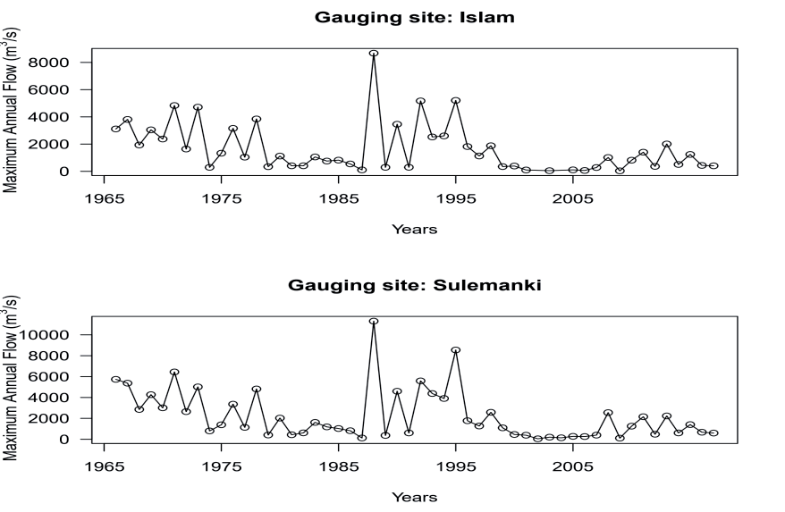
Table 2.
Probability density, cumulative distribution, and quantile functions of the probability distributions.
L-moments Estimation Approach
Pioneered by Hosking [40, 41], the L-moments are computed as direct linear functions of probability-weighted moments (PWM). Although it is a common and easy approach to compute L-moments using PWM [9, 10, 42], L-moments are generally more efficient and convenient compared to PWMs while dealing with practical problems, as they directly quantify the measures of scale and shape of any distribution. For any distribution with quantile function φ(F), the rth PWM Br is theoretically defined as:
For a given set of n sample values x1, x2, x3, ..., xn, the first four PWMs are calculated as:
where x(j) is the jth order statistic in the sample of n observations.
Subsequently, the corresponding L-moments are calculated directly through the following relationships:
As a function of L-moments, Hosking [41] proposed L-coefficient of variation (τ2), L-coefficient of skewness (τ3), and L-coefficient of kurtosis (τ4)as:
λ λ λ τ = 2 , τ = 3 , τ = 4 . 2 λ1 3 λ2 4 λ2
Similar to the method of moments estimation, parameters by the L-moments (LM) technique are estimated in a simple and straightforward way. The solution of the system of equations obtained by matching theoretical L-moments with corresponding sample L-moments yields the estimates for unknown parameters.
Maximum Likelihood Estimation Approach
Maximum Likelihood (ML) is one of the most common methods for estimating the parameters of probability distributions. The principle of the ML approach lies in identifying values that maximize the likelihood or log-likelihood function. Consider a random sample of n observations x1, x2, ..., xn from a probability distribution having a density function f(xj|θ) with θ being the vector of unknown parameters. The ML estimate of θ is obtained by setting the derivative of the log-likelihood function ι(θ) with respect to the elements of θ equal to zero and solving the resultant system of equations. If a closed-form solution is not achievable, numerical optimization techniques can be used to obtain the ML estimates. This study employed the SANN (based on simulated annealing) algorithm for numerical optimization using R-language [43].
Least Squares Estimation Approach
The Least Squares (LS) approach is frequently employed for estimating the parameters of models [44- 46]. In the context of probability distributions, the LS approach minimizes the sum of squared difference between corresponding theoretical and observed CDFs. Algebraically,
where F(xj) and
Weighted Least Squares Estimation Approach
Pioneered by Bergman [47], the Weighted Least Squares (WLS) approach is a modified version of the ordinary LS approach. Unlike the LS method, which applies the same weights to all observations, WLS assigns diverse weights to different observations. These weights are computed through a certain weight function. In the WLS approach, parameter estimation is done by minimizing the sum of squared weighted difference between theoretical and sample CDFs algebraically,
Following the findings and recommendations of different previous studies [48-50], we have used the following function to compute weights to be assigned to different observations:
Relative Least Squares Estimation Approach
The Relative Least Squares (RLS) method, introduced by Pablo and Bruce [51], is another modified form of the simple or ordinary LS estimation approach. Recent findings suggest that RLS performs better for different probability distributions [37, 52, 53]. Unlike the LS approach (which minimizes the sum of squared difference between theoretical and sample CDFs), the RLS approach aims to minimize the sum of squared relative difference between the two CDFs. Simply put, through the RLS method, parameters are estimated by minimizing the objective function given as:
Just like in the case of LS and WLS approaches, numerical optimization techniques can be used in case of complex functions that do not result in unique closed-form solutions.
Performance Metrics
The comparative performance of various potential models is evaluated to recommend the most optimal model (blend of distribution and estimation strategy) for a particular gauging location. The comparison among different competing models is done using commonly applied accuracy metrics (like RMSE, RMSPE, MAE, and MAPE) and p-values associated with some goodness-of-fit (GOF) tests (like KS, AD, and CVM). The test statistics for the GOF tests employed are given as:
Similarly, accuracy measures are defined as:
where Fn(xj) and F̂ (xj) denote the observed and expected CDF of the distribution, respectively. The model with the highest p-value (in the case of the GOF test) and the lowest value (in the case of accuracy measures) is deemed best suited.
After ranking each model based on the above seven performance metrics, a total rank for each model is computed by summing the ranks from these performance indicators as follows:
Finally, for a given gauging location, the model with the highest total rank score is considered the most suitable and optimal model for that particular location.
Estimation of Flood Quantiles
Estimating the maximum flow for a given return period (T) is another vital objective of any FFA. The return period T is generally given in years and indicates how often the peak flow is expected to recur. The estimated flood level xT corresponding to a return period of T years may be defined as the flood of xT magnitude and is expected to exceed once in T years. Thus, the cumulative probability of non-exceedance (i.e., the likelihood that the flood level will not be surpassed in a given year) is:
Now, the value F can be inserted in the quantile function of the most suitable model to estimate flood level xT for return period T. The expressions of quantile functions of different distributions applied in the current study are given in Table 2. The parametric bootstrapping approach [9, 10, 54] is applied to estimate the standard errors of predicted flood quantiles (xT). Based on these standard errors, 95% confidence intervals are also constructed. The parametric bootstrap approach creates a sampling distribution by generating repeated samples from a particular distribution with estimated parameters. This sampling distribution is then used to compute standard errors for the associated parameter estimates.
Results and Discussion
Table 3 presents the summary statistics for annual maximum flow data for gauging sites considered in the current analysis. For any FFA using probability models, the main assumptions about data series are randomness, independence, stationarity, and skewness [10, 17, 55]. In this study, we have used Wald-Wolfowitz (WW), Augmented Dickey-Fuller (ADF), and autocorrelation coefficient (AC) tests to test the validity of randomness, stationarity, and both independence and skewness, respectively.
The outcomes given in Table 4 clearly indicate that these tests confirm that the data series from both gauging sites satisfy the prerequisite assumptions for conducting at-site FFA.
The parameters estimated (with parametric bootstrap standard errors in parentheses) using various estimation methods for candidate distributions are provided in Tables 5 and 6 for gauging sites located at Islam and Sulemanki, respectively. For both gauging sites, each probability distribution and estimation approach combination was ranked based on accuracy measures and p-values associated with GOF tests. The highest p-value (for GOF tests) and the lowest value (for accuracy measures) were given the highest rank. The total rank score, determined by summing all ranks, is used as a single performance measure for identifying the most plausible model for each gauging site.
The results given in Tables 5 and 6 indicate that the generalized Pareto distribution estimated through the WLS method is the most optimal model for both gauging locations considered for the analysis. Moreover, the same probability distribution estimated with the LS and LM methods is found to be the second-best choice for the Islam and Sulemanki gauging sites, respectively. This outcome contrasts with previous research focused on at-site FFA [9, 10, 56] that identified and recommended different other probability distributions as most suitable for various stations of different rivers analyzed therein.
After identifying the most plausible model for a certain gauging location, the next important step in any at-site FFA is estimating flood levels for various return years. These flood quantiles are determined using the selected model’s quantile function and estimated parameters. Table 7 presents the quantile estimates for both gauging locations with certain non-exceedance probabilities (F) for return periods ranging from 5 to 1000 years. The table also provides the standard errors computed through parametric bootstrapping and the resulting 95% confidence intervals associated with the estimated yearly maximum flow. The magnitude of the standard errors for different return years suggests that flood estimates for longer return periods have less precision than those for relatively shorter return periods.
Table 3.
Descriptive statistics of the Sutlej River’s yearly maximal flow (m3/s).
| Gauging location | n | Mean | Median | Maximum | SD | CV |
|---|---|---|---|---|---|---|
| Islam | 50 | 1665.769 | 1048.672 | 8676.99 | 1791.828 | 1.075676 |
| Sulemanki | 52 | 2216.793 | 1260.836 | 11311.25 | 2371.395 | 1.069741 |
Table 4.
Results of testing prerequisite assumptions for data series.
| Gauging location | n | ADF (P-value) | WW (P-value) | AC (P-value) | Skewness |
|---|---|---|---|---|---|
| Islam | 50 | 0.0437 | 0.253 | 0.947 | 1.6396 |
| Sulemanki | 52 | 0.0373 | 0.401 | 0.532 | 1.6397 |
Table 5.
Parameter estimates and ranking of models (gauging location: Islam).
Table 6.
Parameter estimates and ranking of models (gauging location: Sulemanki).
Table 7.
Predicted flood levels for various return years with 95% bootstrap confidence limits.
Conclusions
Modeling of yearly peak flow at two gauging locations of the Sutlej River was conducted using some well-known probability distributions estimated using various estimation techniques. The goal was to identify the most apt combination of distribution and estimation approach for each location. We evaluated the performance of GLO, GUM, REV-GUM, GEV, and GP probability distributions estimated using ML, LM, LS, WLS, and RLS estimation approaches to achieve this goal. The comparison was based on a total rank computed based on the rankings of seven different performance metrics. The model with the maximum total rank was selected separately as the most optimal for both locations.
Based on our results, we recommend the generalized Pareto distribution estimated with the weighted least squares method as most suitable for modeling the peak yearly discharge for both gauging locations of the Sutlej River considered in the study.
The findings of the current analysis of water flow data can be utilized to analyze and predict flood levels, manage water reservoirs, and plan hydraulic structures along the Sutlej River and its surrounding catchment area. The model recommended for analyzed gauging locations may also serve as a valuable potential candidate model for at-site or regional FFA of the Sutlej River or other rivers in nearby regions.