

Introduction
The semi-arid agro-pastoral ecotone represents a transitional zone from semi-arid areas to arid areas, and from agriculture to animal husbandry, and its ecological environment is complex and fragile [1-3]. As a result of climate change and human activities, the agro-pastoral ecotone is facing various environmental challenges, including droughts, soil erosion, water scarcity, and more [4, 5]. Among these issues, water resources have become a particularly prominent challenge, which is related to the variation of top soil moisture (TSM). TSM is a vital factor constraining regional development, with significant spatiotemporal variability [6]. Previous studies indicated that its spatiotemporal distribution was impacted by climate change, and human activities were also undeniably affecting the distribution and quality of water resources [7, 8]. This variability considerably affects water resource management and ecosystem restoration efforts [9]. Therefore, the study of spatial heterogeneity of TSM and its response to environmental factors holds significant implications for regional hydrological research.
TSM spatiotemporal variability exhibits different characteristics in different regions. In humid and semi-humid climate zones, the spatial pattern of TSM significantly correlated with topography under the wetter condition [10]. On a plateau hillside, TSM follows the same spatial pattern along the hill- slope [11]. In tropical regions, the seasonal fluctuations of precipitation and evaporation significantly influence the variability of TSM [12]. In semi-arid areas, the combination of scarce rainfall and high evaporation intensifies the variability of TSM [13, 14]. Climate factors have a significant impact on TSM in the semi-arid agro-pastoral ecotone. Moreover, in the agro-pastoral ecotone, land use also influenced the spatial variability of TSM [15, 16]. Regarding soil moisture in the semi-arid agro -pastoral transition zone, the research [17] primarily focused on the temporal variation analysis of soil moisture, and lacked a comprehensive analysis of its spatial distribution. However, the spatial analysis of TSM in the agro-pastoral ecotone should also be fully considered.
The spatial distribution of TSM is influenced by the combined influence of climate, soil, topography and vegetation type [18, 19]. Different climatic conditions directly determine the intensity of precipitation and evapotranspiration processes. In regions with limited vegetation and arid climates, the correlation between precipitation and TSM is stronger compared to areas with dense vegetation and higher humidity [20]. Drought was also the main influencing factor of spatial patterns in TSM. In some studies, drought indices were employed to predict changes in soil moisture, among which the standardized precipitation evapotranspiration index (SPEI) was found to be effective and readily accessible for forecasting soil moisture fluctuations [21-23]. Penna et al. [24] study on soil moisture spatial variations in sloped topography indicates that slope account for the majority of the soil moisture spatial variation. Different soil types directly impact the retention and permeability of soil moisture. In addition, vegetation dynamics also strongly influence the water-energy cycles in the region [25]. Although some studies had focused on the influencing factors of spatiotemporal changes in TSM [26, 27], the comprehensive effects of climate, soil, and terrain on different vegetation types of TSM in semi-arid agro-pastoral ecotone with diverse vegetation had not been thoroughly studied.
The research about how various factors drive changes in soil moisture across different vegetation types and the impact of interactions between single and multiple factors on soil moisture could contribute to the optimization of water resource management and allocation, enhancing utilization efficiency, while also deepening our understanding of the intricate interactions among climate, vegetation, soil, terrain, and TSM. It provides scientific support for ecological restoration and protection, and offers direction for sustainable soil moisture management, agricultural production, and ecosystem preservation. Therefore, the spatiotemporal changes of TSM in the semi-arid agro-pastoral ecotone and the driving effects of climate, soil, and topography on TSM under different vegetation types need to be explored. Accordingly, the objectives of this study were to (1) decompose TSM and the influencing variables based on Empirical Orthogonal Function (EOF), and characterize the spatiotemporal patterns of TSM; (2) analyze the driving effects of environmental factors on the spatial variations of TSM under different vegetation types based on the geographical detector model (GDM);
(3) explore the driving effects of climate factors and NDVI on the temporal variation of TSM.
Material and Methods
Study Areas
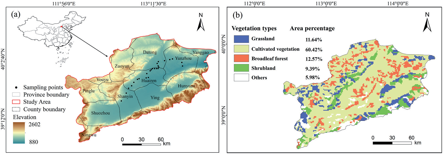
The Sanggan River Basin (SRB) is located in northern China and is situated within the semi-arid agro-pastoral ecotone (Fig. 1a). The annual precipitation was approximately 405 mm and the average temperature was approximately 7ºC over the period 2003-2022. The precipitation in this area is concentrated in summer. The overall topography is low in the middle and high in the south and north. The main soil types are castanozem soil, castano-cinnamon soil, cinnamon soil and fluvo-aquic soil. The vegetation types mainly included cultivated vegetation, broadleaf forest, grassland and shrubland (Fig. 1b).
Data Source and Processing
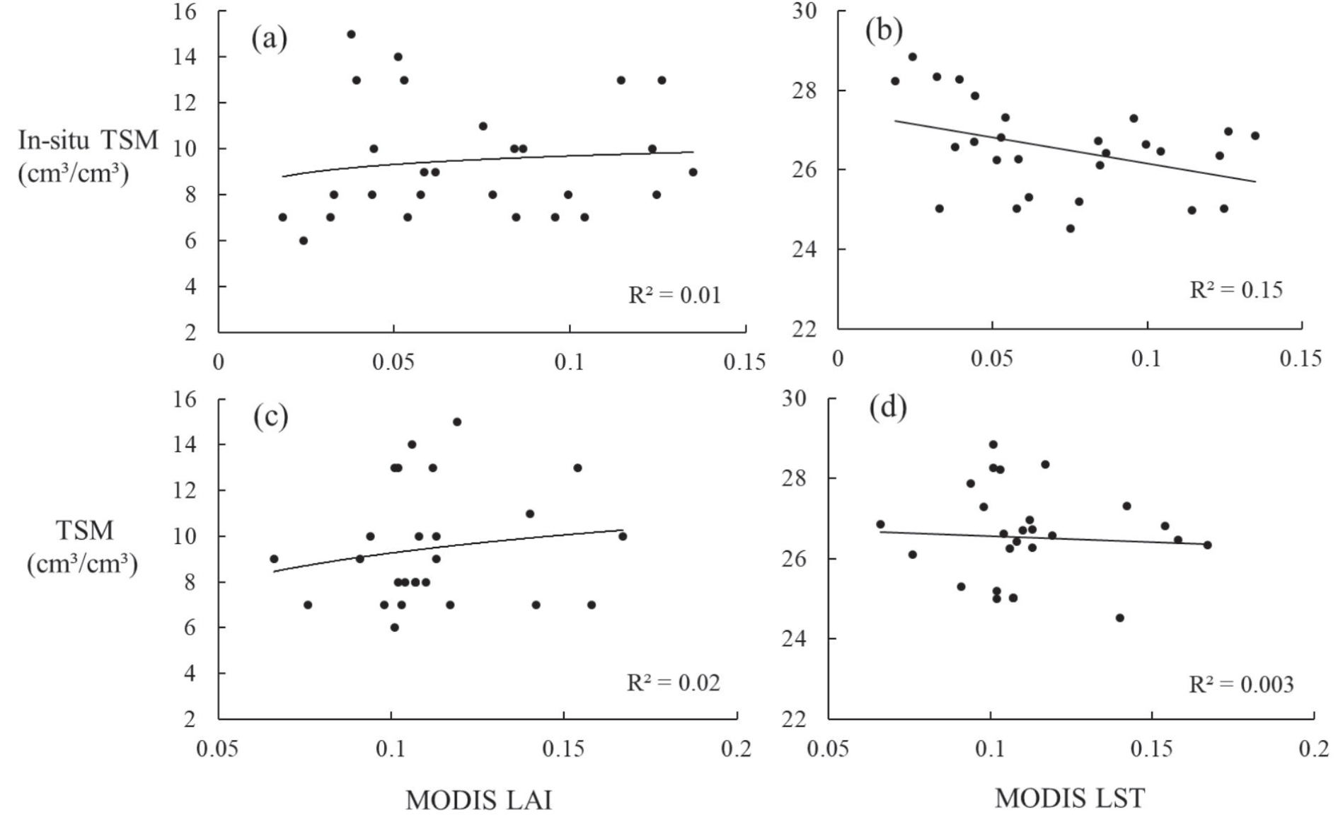
In the study, the in-situ measurements of TSM sampling points were conducted on 11 September 2022 (Fig. 1a). Random locations of 27 samples were selected throughout the entire research area. A 0-10 cm soil sample at each location is taken from the sampling point using a soil auger, subsequently subjected to oven drying at a controlled temperature of 105ºC for a duration of 12 hours, until achieving a state of constant mass. These sampling points were used to verify the validity of downloaded TSM data. Based on the concept of the “Universal Triangle” for validation [28], if the relationship between TSM and MODIS LAI/LST consistent with the relationship between in-situ TSM measurements and MODIS LAI/LST, the TSM data is considered reliable (Fig. 2).
Fig. 1.
Location of SRB and Land Cover Composition and Proportional Distribution of Vegetation Types in SRB.
We have selected a total of 12 representative indicators for factors such as climate conditions, terrain, soil, and vegetation factor, including climate factors such as precipitation, temperature, potential evapotranspiration (PET), SPEI; terrain factors such as Digital Elevation Model (DEM) and slope; and soil factors such as soil organic carbon (SOC), soil bulk density (SBD), sand, silt, and clay content; and vegetation factor such as NDVI. TSM and the climate variables of temperature, PET, precipitation were derived from the National Qinghai-Tibetan Plateau Scientific Data Center with a resolution of 1km (https://data.tpdc.ac.cn/). Based on precipitation and PET, SPEI could be calculated. NDVI was derived from MODIS product MOD13A with 1 km resolution (https://www.earthdata.nasa.gov/). The topsoil texture of SOC, SBD, sand, silt, and clay fractions were derived from the Harmonized World Soil Database (https://www.fao.org/). The DEM with 30 m resolution were downloaded from the ASTER GDEM product, and slope was calculated from it (https://www. earthdata.nasa.gov/). Vegetation types data were derived from the 1:1 million vegetation types in the Data Center for Resources and Environmental Sciences, the Chinese Academy of Sciences (RESDC) (http://www.resdc.cn).
Analysis Methods
EOF Decomposition for TSM
TSM varied greatly at different times and locations, which were controlled by different types of environmental factors. Decomposing TSM into spatial and temporal components to decipher different types of effects are critical to understand its variations, which can be performed by EOF. EOF analysis is a widely applied statistical method for analyzing large multi-dimensional data sets [29]. It can capture the primary trends of variability within TSM data and analyze the spatial distribution and disparities of TSM. This allows us to discern the significance of each pattern in the dataset, thereby focusing on the most representative aspects within the data. With the aid of these patterns, we can identify spatial discrepancies in TSM and reveal the spatial distribution patterns underlying these variations. The EOF was expressed as:
where the left side is the original time series of TSM, and EOF (x, y)i and PC(t)i represent the spatial pattern and temporal component of each mode, respectively. A detailed description of EOF can be found in previous studies [30-32].
Geographical Detector Model (GDM)
Geographic detectors are a spatial statistical method that reveals driving factors by detecting the spatial stratification heterogeneity of elements [33]. They utilize q statistics as a quantitative tool to assess spatial heterogeneity, analyze influential factors, and explore the intricate interplay between various variables. Geographic detectors can determine whether there is an interaction between the two factors, as well as the strength, direction, linearity, or nonlinearity of the interaction, by calculating and comparing the q values of each single factor and the q values after the superposition of the two factors [34]. The principle of them can be expressed as:
where q represents the influence of the factor on the spatial change of TSM. The higher value of q indicates a greater influence. N is the number of samples, and σh2 and σ2 refer to the local variance of TSM within stratum h and the global variance of TSM, respectively. A detailed description of GDM can be found in previous studies [35, 36].
Results and Discussion
Spatiotemporal Variation of TSM
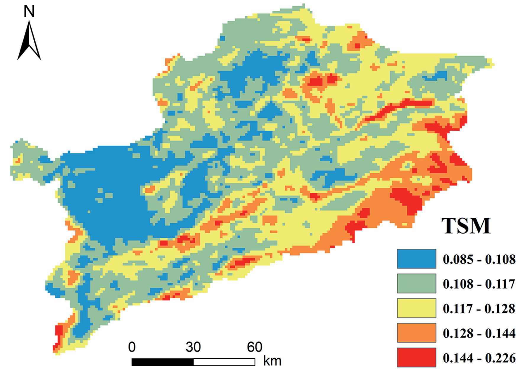
The spatial pattern of TSM was presented in Fig. 3, which decreased gradually from southeast to northwest over 2003 to 2022. Overall, areas with higher elevation tend to exhibit higher averaged TSM values. The areas with high TSM were mainly distributed in higher altitudes on the southwestern and southeastern edges, with vegetation types mainly being grassland and shrubland. The areas with low TSM were mainly distributed in lower altitudes in the center of the watershed, with vegetation types mainly being cultivated vegetation. The TSM of different vegetation types had spatial differences, with shrubland (0.122 / m3·m-3) being the highest, followed by broadleaf forest (0.118 / m3·m-3), grassland (0.116 / m3·m-3), and cultivated vegetation (0.115 / m3·m-3).
Variation of Spatial and Temporal Decomposition
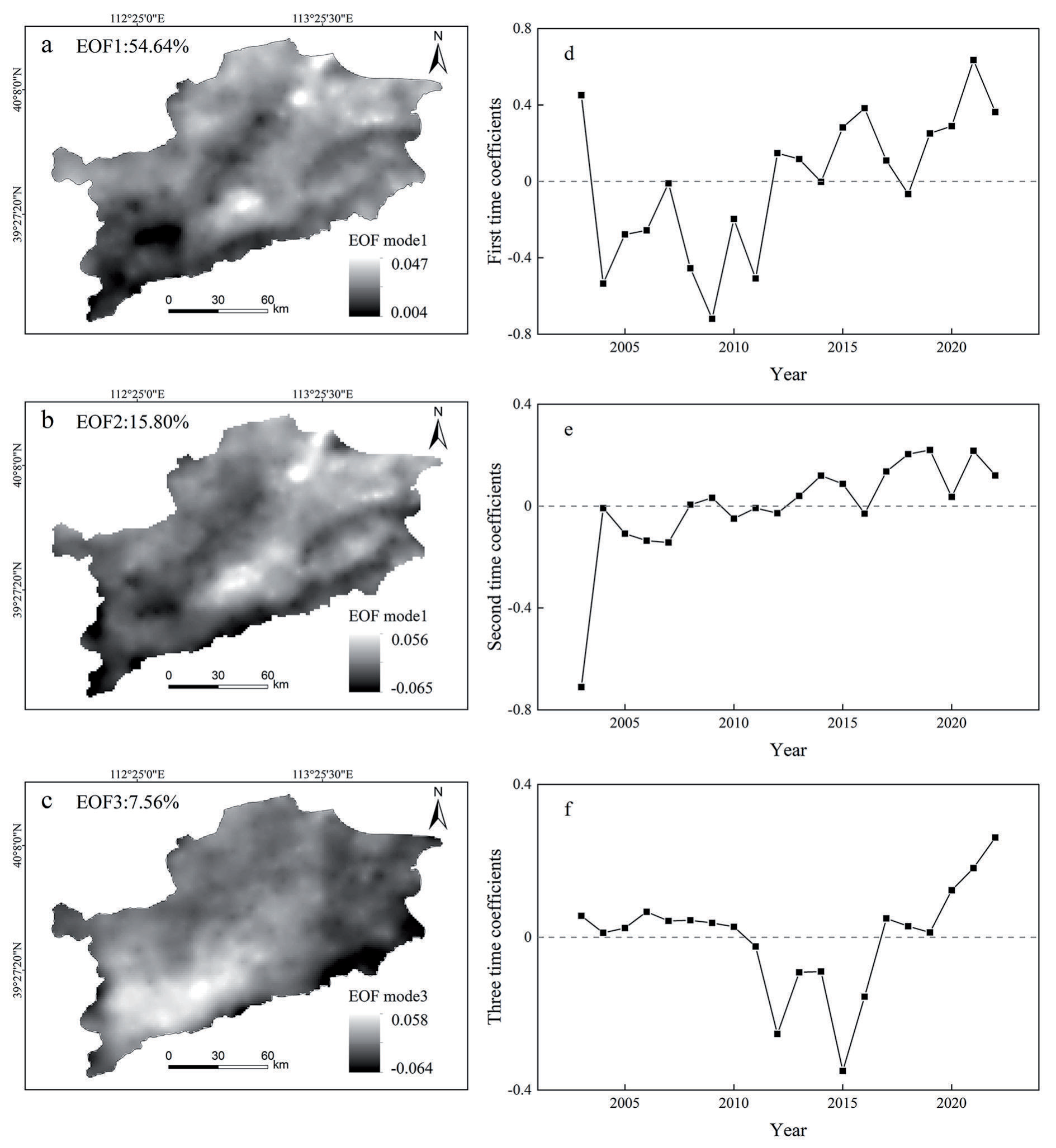
The spatial and temporal variations of TSM over the SRB were decomposed by the EOF. The first three EOFs of TSM were explained 54.64%, 15.80% and 7.56%, respectively, of the total variations of TSM (Fig. 4). They altogether explained 78.00% of the total variation, illustrating that the majority of spatial variability in TSM could be explained by the first three EOFs.
The first EOF mode (EOF1) explained 54.64% of the total variance, which represented the mainly spatiotemporal variability of TSM (Fig. 4a). The values in the first mode were all positive, indicating that the consistency of TSM variability (increase or decrease) in the study area. It is noted that significant variations of TSM were found in the northeast of the SRB and at the junction of Shanyin and Ying County in the central region. The first time coefficient (PC1) showed a large interannual variability (Fig. 4d). From 2003 to 2022, PC1 showed an overall upward trend, indicating an increasing trend in the region, especially in the northeast and central regions. The time series from 2004 to 2011 was negative, and the time coefficient after 2012 was basically positive, reaching the maximum value in 2021. They indicated an “increase - decrease - increase” pattern in TSM.
The second EOF mode (EOF2) explained about 15.80% of the total variance (Fig. 4b). In general, there were similar variation trends in the southwest and in the northeast, with opposite trends in these two zones, indicating that the EOF2 of TSM had regional complexity. The center of the absolute high value was in the southwest, indicating that the TSM changes in the southwest were sensitive. The second time coefficient (PC2) showed a fluctuating upward trend, with a smaller range of changes than PC1 (Fig 4e). PC2 was basically positive after 2013, with a significant increase from 2003 to 2004. This indicates that the changes in TSM in the southwest were relatively sensitive, with sharp TSM changes from 2003 to 2004. After 2008, the overall TSM in the region exhibited a downward trend.
The third EOF mode (EOF3) explained about 7.56% of the total variance (Fig. 4c). The positive center was located in the southwest region, generally decreasing from the southwest to the surrounding areas, while the high center was located in the southeast. The third time coefficient (PC3) was bounded by 2010 and 2017, which were the time points from positive to negative and from negative to positive, respectively (Fig. 4f). This indicated that the southeastern region had experienced a “dry - wet - dry” change.
Effects of Environmental Factors on TSM
The Impact of Influencing Factors on the Spatial Variation of TSM
The correlation between TSM and climate factors and NDVI was presented in Fig. 5. In most regions, there existed a positive correlation between TSM and NDVI, with a more pronounced effect observed in the northern periphery and central valley areas. Broadleaf forest demonstrates the highest average correlation with TSM among different vegetation types, followed by cultivated vegetation, grassland and shrubland. Precipitation and SPEI exhibited a positive correlation with TSM. Increased precipitation contributes to TSM replenishment, and the lower the SPEI value, the drier the region, indicating that drought had an inhibitory effect on TSM. Among different vegetation types, grassland exhibited the highest average correlation between precipitation and TSM, followed by shrubland, broadleaf forest and cultivated vegetation. The highest average correlation between precipitation and grassland may be due to the strongest correlation between precipitation and TSM in areas with limited vegetation [20]. The average correlation between precipitation of cultivated vegetation in the north and east and TSM was low. This discrepancy may arise from human activities, particularly irrigation, which can influence the spatial distribution of soil moisture under farmland and subsequently the relationship between precipitation and soil moisture. Previous studies have demonstrated that human activities constitute the foundation for disparities in the trends of precipitation and soil moisture [37]. At the same time, human activities (i.e., land leveling) will reduce the impact of topography under cultivated vegetation. Shrubland demonstrate the highest average correlation between SPEI and TSM, followed by grassland, broadleaf forest, and cultivated vegetation. The spatial distribution of temperature and Pet correlations with TSM reveals similar patterns. Negative correlations were predominantly found in regions with higher elevation in the southern and western peripheries, while positive correlations were prominent in the northeastern areas. Among vegetation types, cultivated vegetation exhibited the highest average correlation between Pet and TSM, followed by broadleaf forest, grassland and shrubland. Broadleaf forest showed the highest average correlation between temperature and TSM, followed by cultivated vegetation, grassland, and shrubland.
Fig. 4
(a, b, c) the first three leading EOF modes and (d, e, f) their corresponding time coefficients of TSM
Calculate the q values of each factor using a factor detector to quantify its explanation for TSM spatial variation. The greater the q statistic is, the stronger the explanatory power of the influencing factor. Table 1 reveals that precipitation and SPEI were the primary influencing factors of EOF1, exhibiting q values of 0.30 and 0.36, respectively, with an explanatory power above 30%. SPEI, precipitation, DEM, Pet, and slope were the main influencing factors of EOF2. The explanatory power of SPEI and precipitation was above 50%, while the explanatory power of DEM, Pet, and Slope is above 20%. Pet, temperature, precipitation, DEM, and SPEI were the main influencing factors of EOF3. The explanatory power of Pet and temperature was above 30, while the explanatory power of precipitation, DEM, and SPEI was above 20%. Precipitation and SPEI were the main influencing factors on the spatial variation of TSM, which had a significant impact on all three modes after TSM decomposition.
The influencing factors and explanatory power of TSM spatial variation vary among different vegetation types (Table 2). The spatial changes of TSM under different vegetation types were closely related to precipitation and SPEI. Precipitation was the most significant climate factor that influences variation of soil moisture [38]. Precipitation plays a more important role than temperature in explaining changes in soil moisture in arid areas [39]. For the EOF1 of TSM, the explanatory power of DEM, slope, temperature, Pet and NDVI on the TSM of broadleaf forest was significantly higher than that of other vegetation types; Precipitation and SPEI had strong explanatory power for TSM of all vegetation types, but they had the highest explanatory power for broadleaf forest, both above 35%; SOC, clay, sand and silt content all had explanatory power above 10% for grassland, higher than other vegetation types. For the EOF2 of TSM, precipitation and SPEI have strong explanatory power for all vegetation types, with the highest explanatory power for grassland, both higher than 55%; The explanatory power of DEM, slope, temperature, and Pet on the TSM of broadleaf forest was significantly higher than that of other vegetation types; NDVI and SOC had the highest explanations for shrubland, with 0.17 and 0.26, respectively; Clay, sand and silt content all had an explanatory power of over 10% for grassland, which was higher than other vegetation types. For the EOF3 of TSM, DEM, precipitation and Pet had strong explanatory power for the TSM of grassland, all above 30%; The explanatory power of temperature and Pet on shrubland was higher than that of other vegetation, with values of 0.39 and 0.41, respectively; The explanatory power of precipitation, temperature, Pet and SPEI on broadleaf forest was relatively high, all higher than 20%; The explanatory power of each factor on the TSM of cultivated vegetation was relatively low, with Pet having the highest explanatory power at 0.25. The effects of temperature and Pet on EOF2 and EOF3 were more significant than EOF1, which may be related to the concentration of cities and high population density in the southwestern region, where temperature and evaporation had a greater impact on TSM. Human activities exacerbate the urban heat island effect, leading to higher temperatures, which in turn increase the rate of evaporation. In addition, the topography also had a significant impact. Previous studies have shown that TSM increases with decreasing altitude, and depression may also accumulate soil water, leading to the accumulation of soil water [37, 40]. There were also studies indicating that in controlling the spatial variability of regional TSM, soil properties may exceed meteorological forcing [41], and clay content and silt content increase the retaining ability of a soil, which could effectively maintain soil moisture. On the contrary, sand content enhances soil drainage, making it difficult for water to remain in the soil. Therefore, the correlation coefficient between soil moisture and sand content were negative, while clay content and silt content were positively correlated [42]. In addition, the vegetation structure and root distribution characteristics of grassland caused variation of soil texture and have an impact on soil infiltration capacity [43]. In all spatial modes, grassland soil moisture and soil texture show a certain correlation.
Fig. 5.
Spatial distribution of correlations of TSM and a) NDVI, b) Precipitation, c) SPEI, d) potential evapotranspiration and e) temperature in SRB from 2003 to 2022. The null values indicate insignificant correlation (P<0.05).
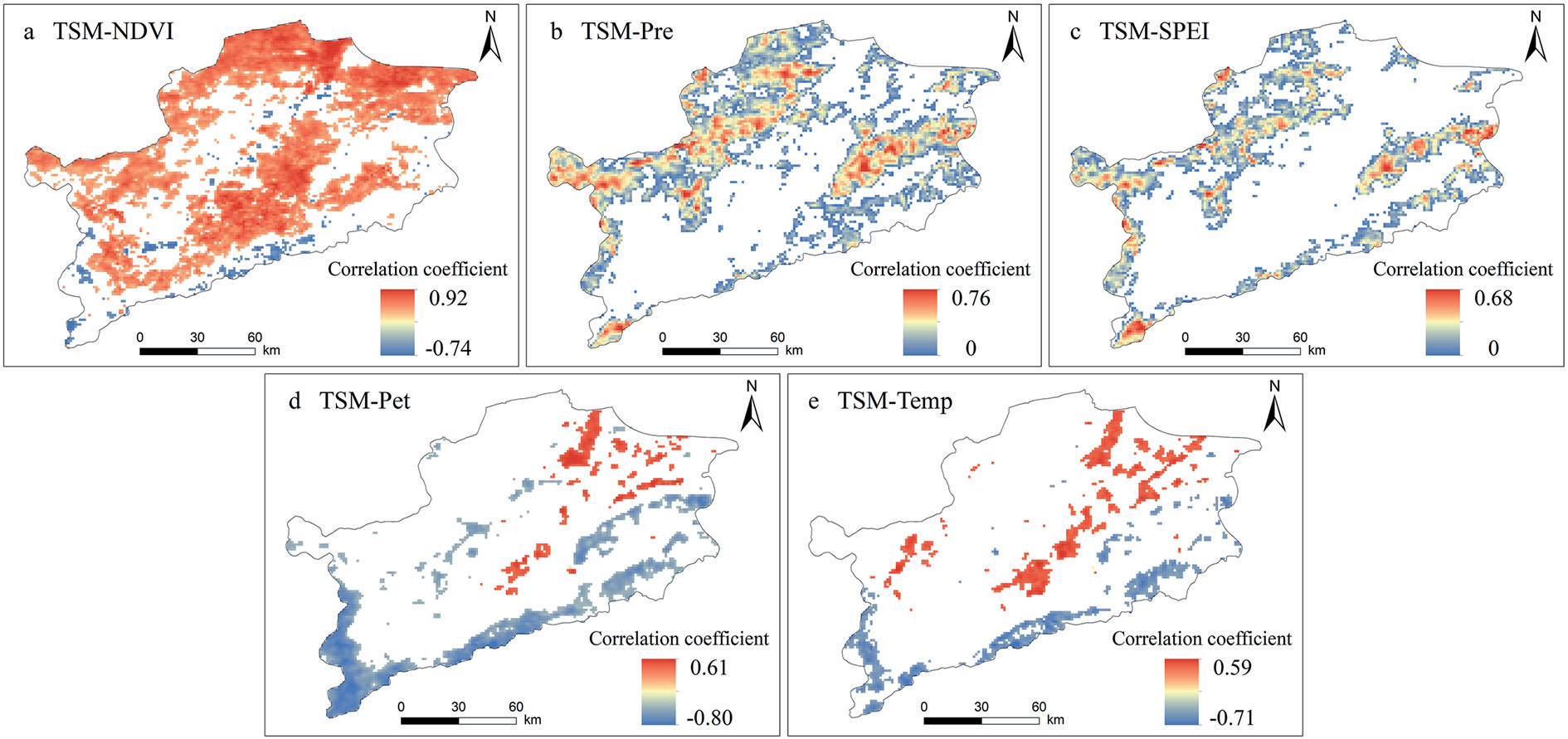
Table 1.
The q values of influencing factors in the first three modes of TSM.
Table 2.
The q values of influencing factors in the first three modes of TSM under different vegetation types.
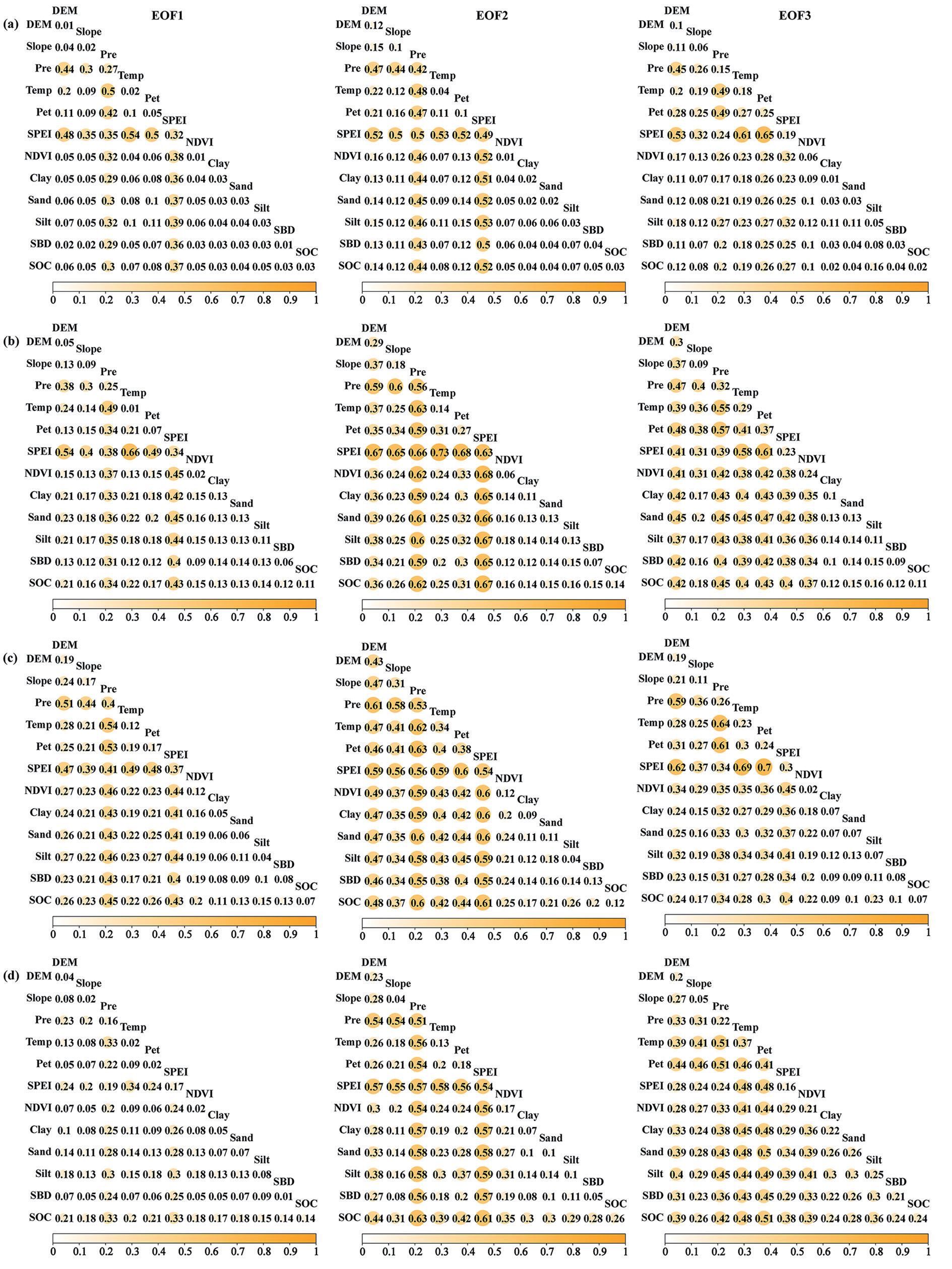
The interaction detection results indicated that the interaction of influencing factors mainly manifests as mutual enhancement and nonlinear enhancement, indicating that the superposition of two factors will enhance the explanatory power of a single factor on TSM spatial variation. . This suggests that the spatial variation of TSM is not solely governed by a single factor but is primarily influenced by a combination of multiple factors (Fig. 6). For the EOF1 of TSM, the interaction between temperature and SPEI had the highest explanatory power for TSM changes, followed by the combination of Pet and SPEI, DEM and SPEI. For the EOF2 of TSM, the interaction between temperature and SPEI had the highest explanatory power for TSM changes, followed by the combination of silt content and SPEI, sand content and SPEI. For the EOF3 of TSM, the interaction between Pet and SPEI had the highest explanatory power for TSM changes, followed by the combination of temperature and SPEI, precipitation and Pet. Although the explanatory power of the soil factor for TSM changes was relatively low, its interaction with other factors enhances its explanatory power, especially when combined with climatic factors. The interaction of the soil factor with precipitation and SPEI had a higher explanatory power for EOF1 of TSM than 30%, and a higher explanatory power for EOF2 of TSM than 50%, significantly improving the explanatory power of the soil factor. The dominant interactions vary among different vegetation types (Fig. 7). Under the type of cultivated vegetation, the combination of factors with the highest explanatory power for the first two modes was temperature and SPEI, while Pet and SPEI had the highest explanatory power for EOF3. The combination of temperature and SPEI had the strongest explanatory power for the TSM changes in the first three modes of grassland. For the first three modes of TSM in broadleaf forest, the combinations of factors with the highest explanatory power were respectively temperature and precipitation, Pet and precipitation, and Pet and SPEI. The combination with the highest explanatory power for the first three modes of TSM in shrubland was temperature and SPEI, SOC and precipitation, and temperature and precipitation, respectively. The combination of various influencing factors enhances the explanatory power of TSM spatial changes, indicating that the spatial changes of TSM were driven by a combination of multiple factors. In this study, the combination of precipitation, SPEI, and other factors significantly improved the explanatory power of TSM spatial changes, especially when combined with temperature and Pet. The spatial variability of TSM was more influenced by the comprehensive effects of climate factors. The combination of DEM, NDVI, and climate factors had also improved the explanatory power of different vegetation types, especially grassland and broadleaf forest.
Fig. 6.
The interactive effects among factors on the first three modes of TSM, including a) EOF1, b) EOF2, c) EOF3. Notes: Pre (Precipitation), Temp (Temperature), Pet (Potential evapotranspiration), SPEI (Standardized Precipitation Evapotranspiration Index), SBD (Soil Bulk Density), SOC (Soil Organic Carbon).
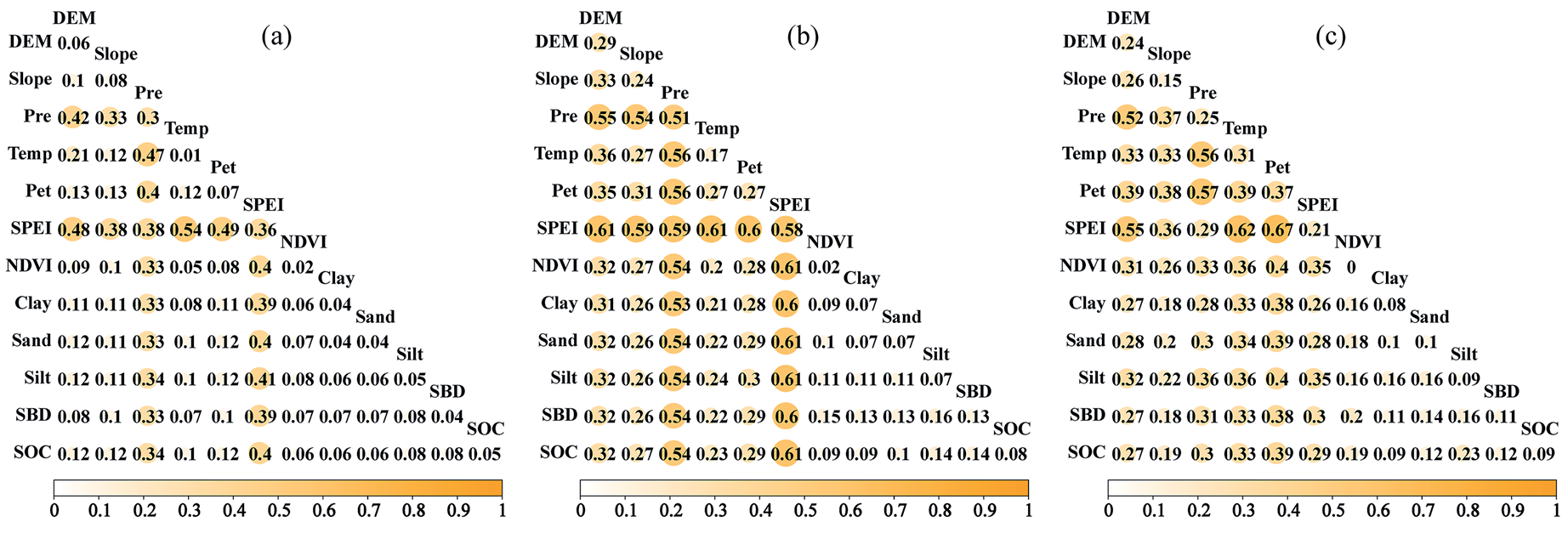
Fig. 7.
The interactive effects among factors on the first three modes of TSM under different vegetation types, including a) cultivated vegetation, b) grassland, c) broadleaf forest, d) shrubland. Notes: Pre (Precipitation), Temp (Temperature), Pet (Potential evapotranspiration), SPEI (Standardized Precipitation Evapotranspiration Index), SBD (Soil Bulk Density), SOC (Soil Organic Carbon).
The Impact of Influencing Factors on the Temporal Variation of TSM
Interannual changes of TSM and temperature, precipitation, Pet, SPEI, NDVI in Fig. 8. The TSM showed a fluctuating upward trend. The interannual changes in temperature and Pet were not significant and showed a fluctuating upward trend. In 2005, 2009 and 2011, the precipitation in the region was low, and the Pet and Temp were high, so it was relatively dry, which had a significant impact on TSM and resulted in lower TSM values. The high values of TSM in 2003, 2013 and 2016 were significantly affected by precipitation. NDVI showed a fluctuating upward trend between 2001 and 2020, which was related to changes in TSM.
In order to study the influence of environmental variables on the temporal variation of TSM under different vegetation types, correlation analysis was performed on the first three PCs of TSM and the environmental variable PC1 (Table 3). Due to the fact that the first mode of climatic factors was both explained above 95% of the total variance, and that of NDVI is above 75%, they already capture the major variations of SRB. Therefore, the analysis will be conducted using PC1 of the environmental factors. Precipitation and NDVI were significantly positively correlated with the PC1 of TSM, while Pet, temperature, and NDVI were significantly positively correlated with the second time coefficient of TSM. This indicated that precipitation and NDVI were important factors affecting the temporal variation of regional soil moisture, and precipitation was one of the main sources of soil moisture. Both exhibited similar interannual variation characteristics, with a decrease in precipitation leading to drought and, to some extent, causing a decrease in TSM. Vegetation has an important impact on the temporal variation of soil moisture, and its growth increases the demand for water, which may lead to the decrease in soil moisture. In addition, temperature could affect the evaporation of soil moisture, thereby affecting the temporal variation of soil moisture.
Fig. 8.
Interannual changes of TSM and a) precipitation, b) temperature, c) potential evapotranspiration, d) SPEI, e) NDVI in SRB from 2003 to 2022.
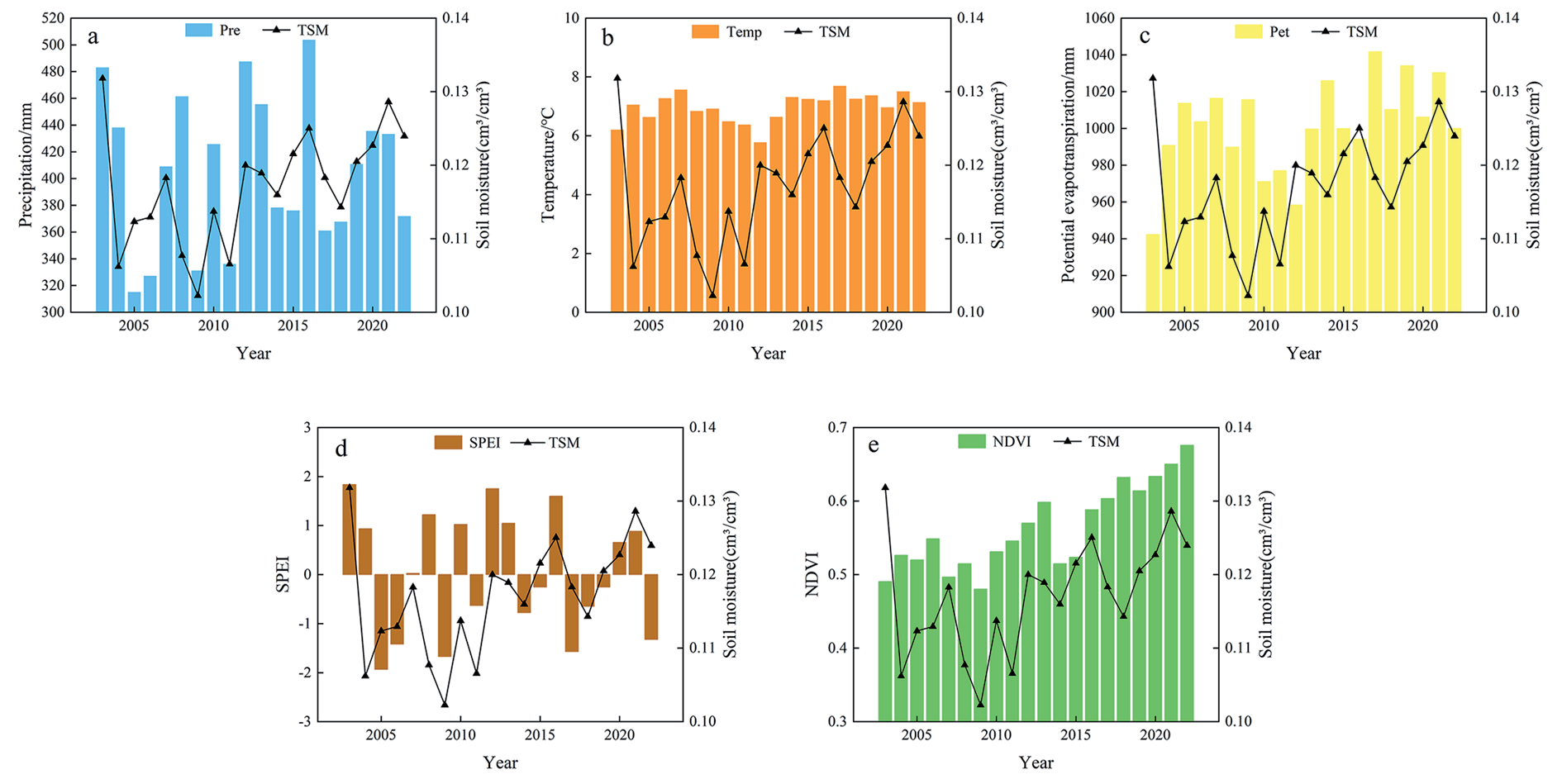
Table 3.
Correlation analysis of time coefficients of climatic factors, NDVI, and TSM.
| Time series of SM | Temp | Pet | Pre | SPEI | NDVI |
|---|---|---|---|---|---|
| 1 | 0.181 | 0.055 | 0.454* | 0.334 | 0.581** |
| 2 | 0.503* | 0.687** | -0.263 | -0.322 | 0.562** |
| 3 | 0.267 | 0.243 | -0.212 | -0.247 | 0.330 |
The temporal variability of soil moisture was closely related to climate factors and NDVI. There is a significant positive correlation between precipitation and the PC1 of TSM. Precipitation was the main source of soil moisture, and the interannual changes of precipitation and TSM have similar characteristics, indicating that precipitation had a significant impact on the temporal changes of soil moisture. Temperature could affect the evaporation of soil moisture, thereby affecting variability of soil moisture. Therefore, temperature and evapotranspiration were also important factors in the temporal variation of soil moisture. Climate factors explain more about the temporal variation of TSM, especially precipitation [34]. In addition, there is a high correlation between the temporal variation of NDVI and TSM, and vegetation cover was an important factor affecting the temporal variability of soil moisture. Higher NDVI values were usually associated with sufficient soil moisture, while lower values indicated drought or insufficient moisture. Research has shown that in the time domain, changes in soil moisture typically occur one month before changes in NDVI, with the positive impact of increased soil moisture promoting plant growth and ecosystem recovery [44].
In summary, our results explored the spatiotemporal changes of TSM in the semi-arid agricultural pastoral ecotone and the driving effects of climate, terrain, and soil on TSM. This is of great significance for the management of water resources in the agricultural and pastoral ecotone in the future, and contributes to the allocation and management of regional water resources. However, our research still has some limitations, such as the impact of human activities within the study area: ecological engineering and artificial irrigation, which have not been taken into account. For example, excessive exploitation of water resources could reduce regional groundwater resources [45], thereby affecting surface water; The construction of ecological engineering, such as the “Grain for Green” program on the Loess Plateau, had an impact on the dynamic changes of soil moisture [46]; Artificial irrigation will restore the upper soil moisture to a certain extent [47]. Therefore, further research is needed to elucidate the comprehensive impact of various factors such as nature and humans on TSM.
Conclusions
This study explored the spatiotemporal changes of TSM in the semi-arid agro-pastoral ecotone and the driving effects of climate, terrain, and soil on TSM. Spatiotemporal patterns of TSM were analyzed using EOF, and the decomposed patterns, based on GDM, were utilized to explore the impact of the single and multiple factors on different vegetation types of TSM.
(1) Climate factors were the main influencing factors on the global spatial variation of TSM, while topography and soil texture had an impact on local spatial changes in TSM. The impact of various factors under different vegetation types varies. Climate factors had a more significant impact on broadleaf forest compared to other vegetation types, with soil texture having a greater impact on grassland and topography having a smaller impact on cultivated vegetation.
(2) The influencing factors did not independently affect TSM, but rather a combination of multiple factors. The interaction of influencing factors mainly manifests as mutual enhancement and nonlinear enhancement. The impact of combined factors was greater than that of a single factor, among which the combination of climate factors had the strongest explanatory power for the spatial variability of TSM. The combination of temperature and SPEI had a stronger explanatory power for the TSM under cultivated vegetation, grassland and shrubland, while the combination of temperature and precipitation had a stronger explanatory power for the TSM under broadleaf forest.
(3) Precipitation and TSM exhibit similar interannual variations, and there was a significant positive correlation between precipitation and NDVI with the temporal variation of TSM. Thus, precipitation and NDVI were the most important factors affecting the temporal variation of TSM.