

Introduction
Rocks under high ground stress are in triaxial compression equilibrium, or limit equilibrium, and store a large amount of energy. The unloading process of underground tunnel excavation will inevitably lead to the redistribution of peripheral strain and the concentration of local strain. When it reaches the ultimate strength of the rock, it will fail. If the energy in the rock is greater than the energy used to destroy the rock, then the remaining energy is released as kinetic energy, ejecting the broken rock to form a rock blast. This is the so-called rock blasting phenomenon, which is a kind of geological disaster in areas with high ground stress. With the extensive construction of traffic tunnels, rockburst has become more and more common in the construction of traffic tunnels, and even become the main technical bottleneck [1-9]. In the field of traffic tunnels, especially in high ground stress areas, there are thousands of engineering accidents caused by rock bursts every year, with approximately 1000 casualties. Many construction projects have been delayed for six months or even longer, and even hundreds of millions of yuan worth of mechanical equipment have been scrapped. Therefore, it is particularly important to explore an efficient and real-time monitoring method for rock bursts [10]. Fig. 1 shows the structural damage and disease caused by the rock burst in the traffic tunnel.
Rock burst is induced by the change of the external environment and stress field, which is a kind of instability result of dynamic rock failure, such as the initiation, development, and penetration of microfracture. According to the characteristics of this process, a variety of methods have been developed to monitor rock bursts. According to the monitoring information, taking measures before a rock burst can ensure the safety of construction. Commonly used methods include the microseismic monitoring method, the acoustic emission method, the electromagnetic radiation method, the rebound method, etc.
(1) Acoustic Emission Method [11-15]
The acoustic emission method is realized by elastic waves generated when cracks appear in rock mass. The acoustic emission signals generated by rock cracks are collected by electronic sensors stored, and analyzed by the system after being amplified by amplifiers.
(2) Infrared Thermography [16-18]
There is an obvious phenomenon of heating during the process to rock failure, and an abnormal change in infrared temperature indicates a fracture. In the excavation, infrared anomalies caused by the rapid rise of the temperature of the surrounding rock are precursors of rock bursts. Infrared thermography technology predicts the possibility of a rockburst by monitoring the thermal radiation temperature.
(3) Electrical Radiation method [19-23]
The electromagnetic radiation signal before a rock burst is obviously abnormal. The occurrence of a rock burst can be predicted well by monitoring the abnormal electromagnetic radiation signal. The electromagnetic radiation monitoring can reflect the stress state of the orebody in time and has the characteristics of non-contact and regional monitoring, which is effective in predicting the rock burst. In addition to the above methods, there are photoelastic methods and deformation methods, which mainly use parameters such as stress, deformation, and damage to infer the occurrence or grade of a rock burst. However, it is difficult to ignore the corresponding limitations when applied to traffic tunnels. First of all, most methods can only monitor the rock mass in a small area, such as the AE method and the infrared thermography method, which cover very limited areas. Secondly, the real-time performance and high efficiency of monitoring methods such as the infrared thermography method and the rebound method cannot be guaranteed. Moreover, such as infrared thermography, electrical radiation methods, and other related technology, research still requires development in the application of specific projects and needs further research. Based on this situation, this paper introduces microseismic monitoring technology with wider coverage, higher timeliness, and more mature technology, and discusses its application in traffic tunnels.
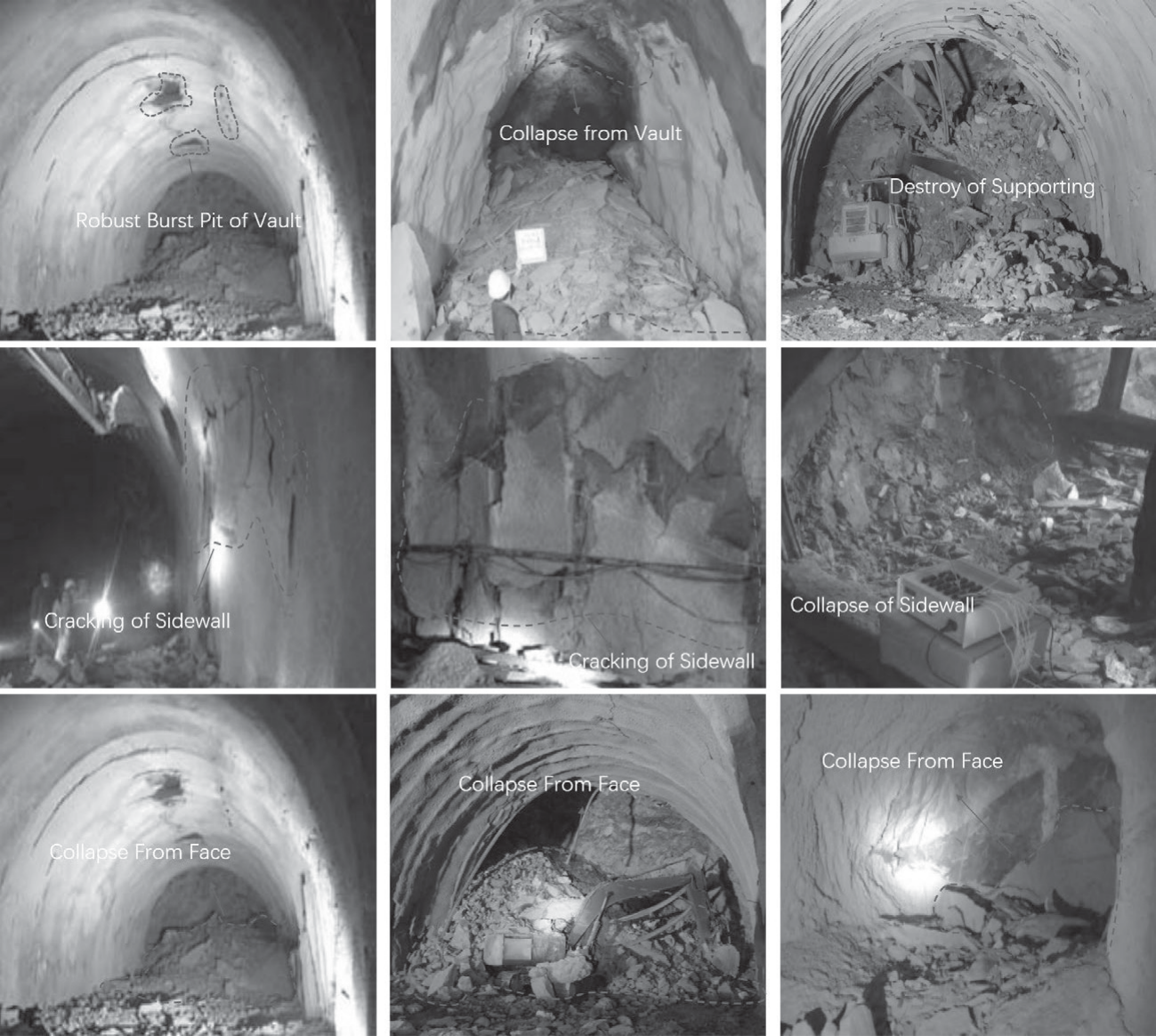
Table 1.
Different rock burst monitoring methods.
At present, microseismic monitoring has been applied to mining tunnels, hydraulic tunnels, etc., and has been proven to be able to monitor the occurrence of rock bursts during tunnel excavation in real time and successfully warn [24-26]. In traffic tunnels, the application of microseismic monitoring is not yet mature. In this review, the specific process of microseismic monitoring will be introduced by comparing the differences between mining tunnels and traffic tunnels.
Microseismic Monitoring
Conventional monitoring of rock bursts is always not so continuous, not real-time, and difficult to detect the instantaneous change. These problems were all crucial in the monitoring of rock bursts. Microseismic monitoring has been proposed to solve these problems. Microseismic monitoring determines the stability of the rock and the chance of a rock burst by the signals generated when fractures happen. With the boom of computer technology and advanced algorithms, microseismic monitoring has been well developed in geotechnical and tunnel engineering, including mining engineering [27], hydropower copper chamber [28], tunneling engineering [29], rocky slope [30] and other projects.
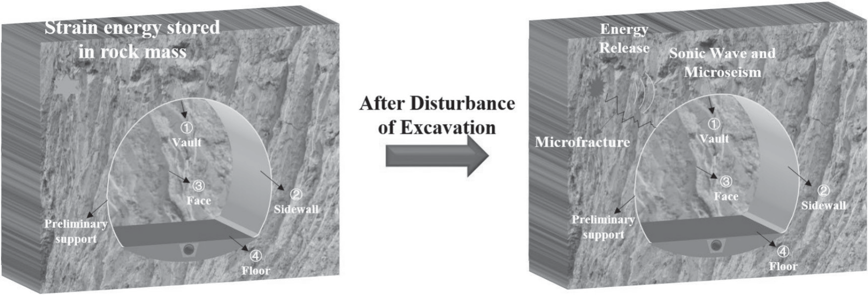
Fig. 2 is a schematic diagram of the application of microseismic monitoring in tunnels. When rocks are subjected to ground stresses, local concentrations of elastoplastic energy occur. And when the energy accumulates to a critical value, it will lead to the creation and propagation of microcracks in the rock, releasing energy in the form of elastic or stress waves. Microseismicity is a phenomenon that accompanies the process of rock destruction. Microseismicity contains a wealth of information about the damage and geological activation processes in the surrounding rocks [31-34]. A reasonable and scientific arrangement of some pickups in the monitoring area to collect the microseismic signals can infer the internal morphological changes of the rock and its damage mechanism. Microseismic monitoring is developed based on seismic monitoring. The principle of it is the same as seismic monitoring and acoustic emission monitoring technology, basically. In contrast, the advantages of microseismic monitoring are greater; in particular, microseismic monitoring has a wider signal frequency and a larger monitoring range than acoustic emission monitoring. When it comes to the actual application, a proper microseismic monitoring system must be selected to meet the needs of rock blasting monitoring, that is, to be able to cover the frequency range of the breeding process of rock burst.
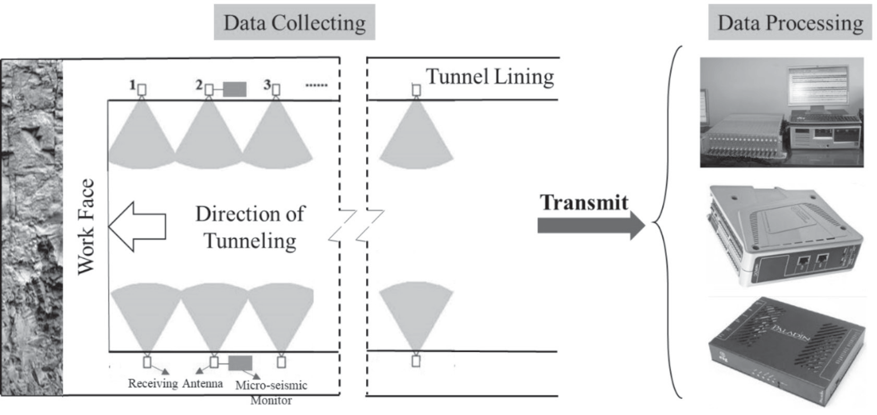
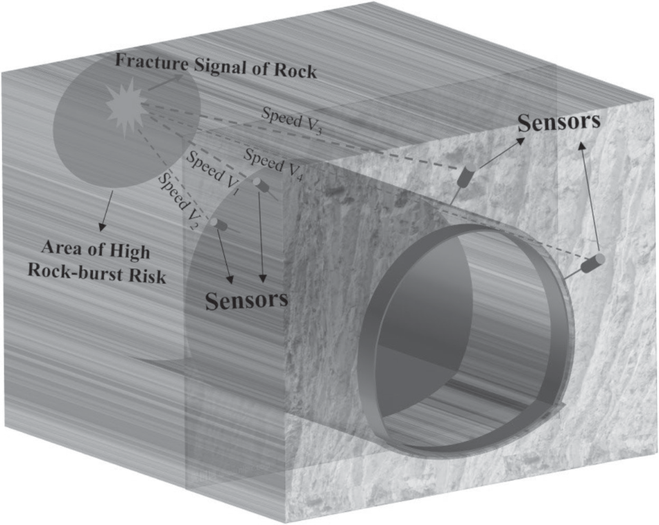
The tunneling will increase local microcracks, which could lead to microcracks in certain areas, forming areas of agglomeration, or severe damage, as shown in Fig. 3. The energy from the disturbance of the tunnel envelope will propagate in the form of vibrations and sound waves in all directions and be received by multiple sets of pre-planted geophones. Since the distance between the source and the geophones is varying, the time taken for the vibration wave to propagate to the geophones and the arrival times accepted on the geophones will also vary. The localization of the source and the calculation of the energy can be carried out based on the differences in arrival time between the individual geophones. The location and energy of this rock rupture can be displayed in a three-dimensional space. Microseismic monitoring of rock bursts is based on the assessed source. Multiple sensors are arranged to collect elastic wave signals released from the rupture of the rock in the area of the rock burst. Based on these signals, further analysis can be carried out to obtain the location, time, energy, etc. of the rupture. On this basis, rock movement, mathematical statistics, fuzzy mathematics, simulated annealing-simple shape algorithm, moment tensor, fractal mathematics, and the double difference localization method are also used to study the active characteristics of predicting and forecasting the dynamic disaster of a traffic tunnel under high ground stress.
Microseismic monitoring has shown its advantages in many applications. These include three-dimensional spatial monitoring with a large range, a continuous monitoring process, timely and intuitive processing and analysis of monitoring results, being less labor-intensive, and the ability to transmit data over long distances. Feng et al. studied the microseismic characteristics during the development process of rockburst and analyzed the mechanism of rockburst formation [35]. Zhang et al., based on the rockburst process of the Jinping II hydropower station, found that the microseismic monitoring process has a sleep period, which can be used to evaluate the development process and laws of rock bursts [36]. Although traffic tunnels and mining tunnels have some differences in many aspects, the advantages of microseismic monitoring are still effective when applied to traffic tunnels. The deference mainly includes the section size, construction methods, and operating conditions. The main issues that require addressing when using microseismic monitoring to detect rock bursts in traffic tunnels under high ground stress are signal acquisition and source location. However, there are still several issues that need to be considered in the application, especially the difference between traffic tunnels and mining tunnels.
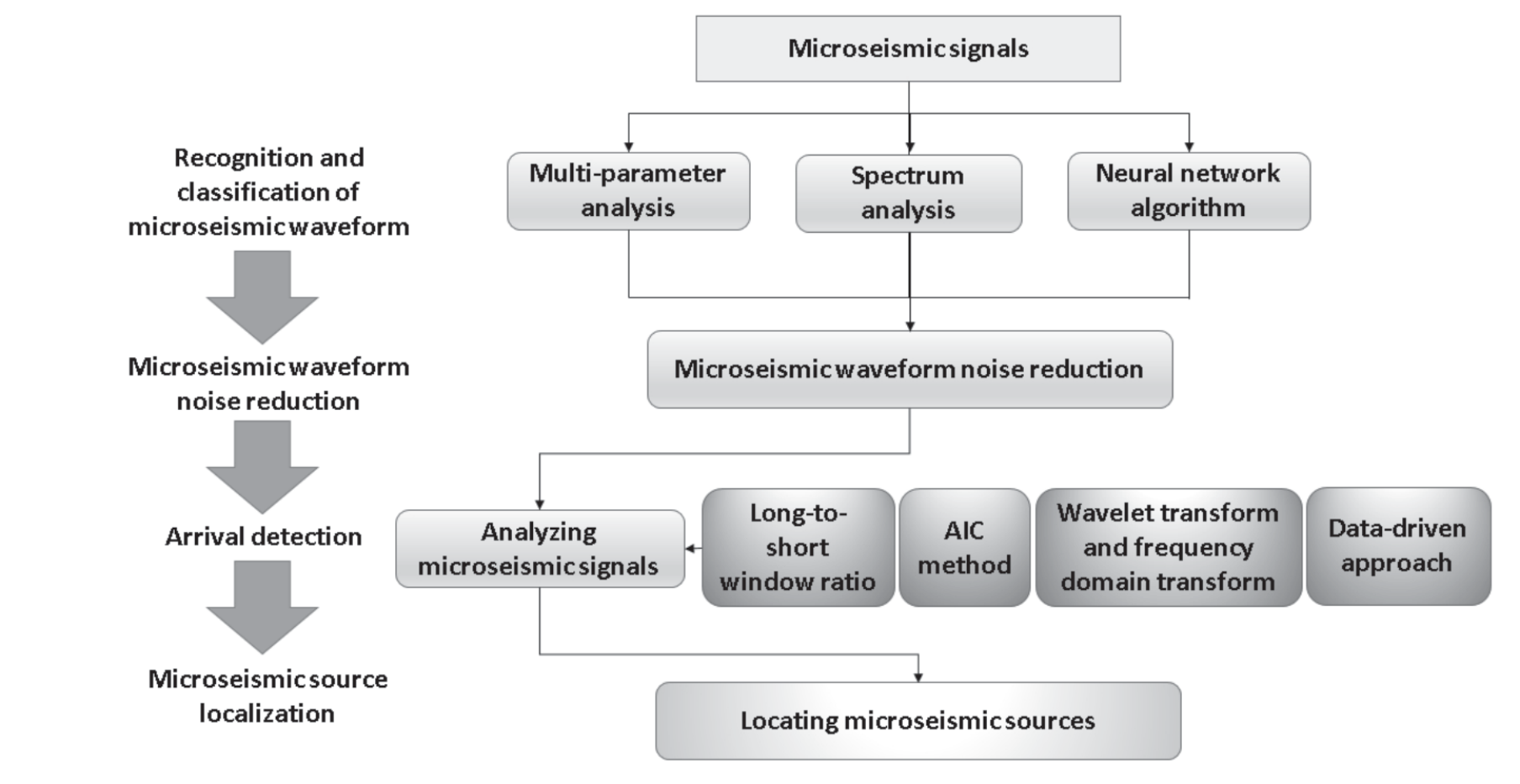
Firstly, in terms of signal acquisition, the considerations of the arrangement of sensors are different. Mining tunnels are usually not very large in cross-section, so the area that needs to be considered is not as large as a traffic tunnel. However, a certain amount of analysis is still required to ensure the signals are adequately received in the risk area of rock burst within the excavation when the section size increases exponentially. Secondly, in terms of signal recognition and classification, due to the much larger scale of traffic tunnels compared to mining tunnels, the areas affected and interfered with by signals will also expand, leading to difficulty in signal recognition and unclear classification. At the same time, during the construction period, the deformation of the traffic tunnel will be strictly controlled through advanced support and other means, which will also lead to differences in the scope and requirements of microseismic monitoring. Finally, the requirements for signal processing differ in terms of noise reduction and time of arrival detection during signal acquisition. Due to their larger cross-section and higher construction noise, traffic tunnels undoubtedly require higher processing algorithms when real-time and accurate processing of large amounts of information is required. Therefore, it is necessary to discuss in detail the process of microseismic monitoring to explore its application in traffic tunnels. The process of microseismic monitoring can be simply represented by Fig. 4.
Microseismic Monitoring Processes
Signal Acquisition
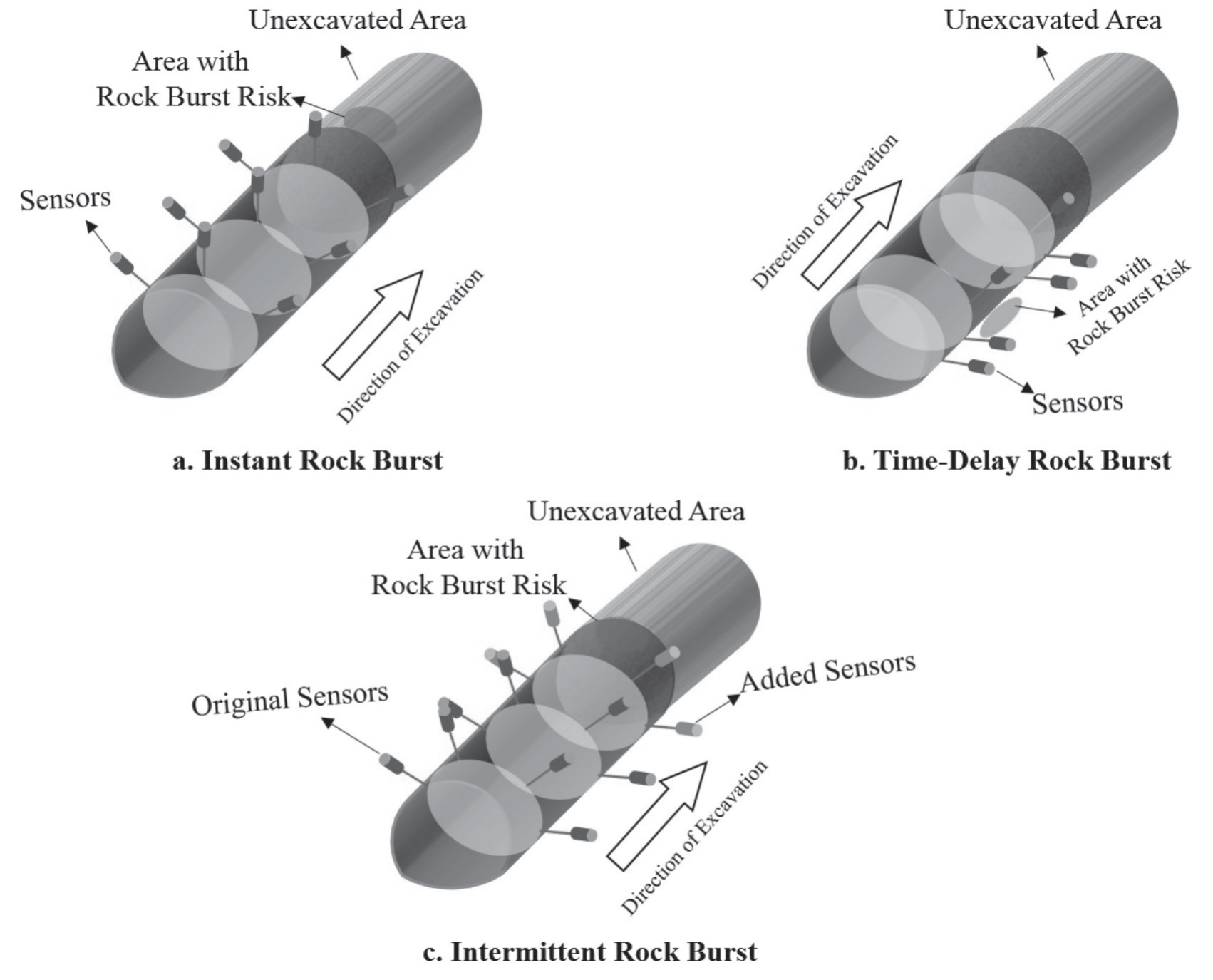
The acquisition of microseismic signals is the basis of microseismic monitoring, and the reasonable arrangement of microseismic monitoring sensors is the basis for effectively capturing rock fracture signals. Different ways of distributing the geophones have different influences on the positioning accuracy. Firstly, the sensor layout should surround the area with a high probability of a rock burst. As shown in Fig. 5a), it is a diagram of the three-dimensional staggered arrangement of sensors in space when a tunnel sensor is unable to surround the risk region of a rock burst. At the same time, the arrangement should be designed according to the area and type of potential risk of a rock burst. And as to the other characteristics, construction methods and conditions should also be considered. Before excavation, sensors should be placed in areas with a high risk of rock burst as close as we can. And during excavation, sensors should be added dynamically to areas of unfavorable geological conditions and areas of high risk of rock burst in close proximity to the excavation process. Sensors should be placed close to potential risk areas of rock burst to effectively improve their ability to capture signals. But consideration should be given to the feasibility and convenience of sensor placement under different construction methods, such as drill and blast construction. Consideration should be given to blasting, which may cause damage. During the TBM construction, consideration should be given to the structure of the TBM when choosing the location for installation. Considering that sensors are usually arranged in groups on the axis, typical sensor arrangements for different types of rock blasting monitoring are shown in Fig. 5. As to an instantaneous rock burst, the sensors should follow the excavation of the face and move dynamically to ensure that the rupture near the face can be captured in real time, as shown in Fig. 5a). For time-lag rock bursts, sensors can be arranged around the potential area of occurrence, as shown in Fig. 5b). For intermittent rock bursts, as the process is usually long and the tunnel is suspended, additional sensors should be temporarily added close to the area of the burst. A typical arrangement for intermittent monitoring of rock bursts in drill and blast tunnels is shown in Fig. 5c).
In optimizing the distribution of geophones, reference should be made to the theories of the optimal distribution of seismic networks. Noureldin et al. [37]. considered the theory and proposed a Monte Carlo algorithm for the numerical calculation of the monitoring capacity of seismic networks and a method for the design of microseismic networks based on D-value and C-value optimization design theory. D-value optimal design theory suggests that the optimization of geophone locations depends on the covariance matrix of the source parameters, and C-value optimal design theory analyzes the relationship between the distribution of the network and the number of conditions in the resulting set of equations from the point of view of the robustness of the affected non-linear system. Guided by the D-value optimal design principle, Gong et al. [38, 39] applied the D-value optimization design theory to design a station network deployment optimization and evaluation system for microseismic monitoring of mine caves and to establish an objective function for the optimal layout of the station network for the large-scale station layout combination optimization problem. In order to be more in line with engineering practices, Toledo et al. [40] designed and characterized local and regional microseismic monitoring arrays dedicated to geothermal exploration and volcano monitoring based on D-value optimization design and finally calculated the location of microseismic occurrence through multiple Monte Carlo experiments. Zhou et al. [41] proposed a network optimization method based on the geometric parameters of the sensor point database, and through the comparison with the existing layout scheme and numerical simulation, it was concluded that the optimization effect of the method meets the engineering requirements for high efficiency and intelligence in signal reception and acquisition.
Recognition and Classification
Data processing is the next step after signal acquisition, and Fig. 6 shows a flowchart of the process of processing the signal after acquiring it. It is a challenge to process the large amount of data collected by the microseismic monitoring system quickly and efficiently. Especially the part to extract and separate the microcapture signals from the noisy signals, which are of widely varying quality. It would be particularly inefficient if they were mainly carried out by experience. Microseismic monitoring techniques are derived from theories based on acoustic emission and seismology [42]. Therefore, the methods of processing microseismic signals in traffic tunnels can be referred to as the processing of acoustic emissions and seismic signals. The process generally consists of four steps: identification and classification, noise reduction, arrival detection, and source localization. The identification of rupture signals is finished by analyzing the microseismic waveform to identify the microseismic events. In the process of signal processing, the signals of rupture and noise often have a similar and intertwined waveform that needs to be processed for noise reduction. The final step in the processing is to locate the source of the seismic activity and determine its exact location, which gives preparation for early warning and prediction.
The first task of signal processing is to identify the microseismic event. It is the fundamental part of the whole process, and if there is an error in this part, the results will be meaningless. The data collected by microseismic monitoring systems is complicated, and most of it is noisy data, which interferes with automatic detection. Therefore, how to extract the microseismic signals accurately and efficiently from the huge amounts of data is a critical issue. There are a lot of studies that have explained the difficulty of distinguishing between microseismic and non-microseismic signals and made remarkable progress on it. The methods of these studies mainly include multi-parameter analysis and spectral analysis.
Multi parameter analysis can use the methods of maximum likelihood, Fisher classification, Bayes discriminant, and logistic regression for microseismic classification and parameter identification. It can extract the relevant features well enough to provide good microseismic detection. However, the variability and complexity of characteristic parameters make this process difficult and inefficient. Spectral analysis has been well used in the identification and classification of microseismic signals because of its simple, rapid, and effective feature extraction [44]. In recent years, the rapid development of various automatic microseismic recognition and classification algorithms has made an important contribution to addressing the inefficiency of microseismic recognition. Some of the classical recognition and classification methods include the amplitude-based long-short window method (Short Term Average/Long Term Average, STA/LTA), waveform correlation, fingerprinting, similar thresholds, etc. Each method has its own advantages and limitations. Mitchell Withers [45] found that an STA/LTA-based signal recognition approach provided the most globally relevant output - based on an event detection and localization system. The STA/LTA method uses the ratio of STA to LTA to represent the amplitude and frequency change of the microseismic signals. The arrival of the signal will cause a sudden change in the value. When the ratio of STA to LTA is greater than the set threshold, it is considered a microseismic event. This method is very effective for high SNR signals, but poor for low SNR signals and easy to miss. Robert J. [46] applied waveform correlation analysis to study matching templates for an earthquake in Ohio and found that waveform correlation analysis works better when microseismic events of the same source mechanism are in the same region, but it requires a high number and quality of templates. An increase in the number of templates can lead to a rapid increase in computational effort, so finding a balance between the number of templates and computational effort is also necessary for fast and effective identification of microseismic events.
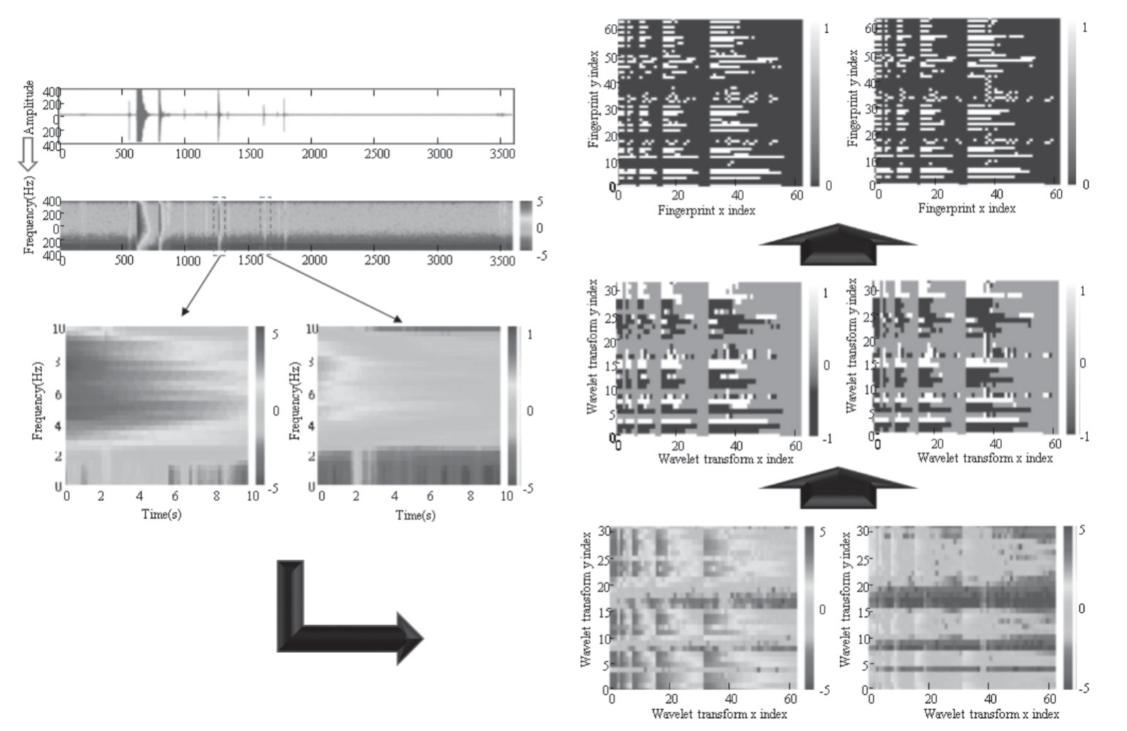
Although the parameter analysis method, spectrum analysis method, and various automatic identification methods are effective. Each method has disadvantages: complex parameters, huge calculations, low efficiency, and instability, for example. With the development of computers, machine learning, and deep learning, recognition methods based on deep learning have been applied to the recognition of microseismic signals at present. The method takes the original waveform as input for identification. It realizes the real-time identification of a large number of microseismic waveforms accurately and efficiently. Yoon et al. [47] developed an effective method for seismic detection using waveform similarity to overcome the shortcomings of existing detection methods, called Fingerprint and Similarity Thresholding (FAST). The Fingerprint and similarity threshold method (FAST) is an audio fingerprint algorithm based on Wave print, which is also a combination of computer vision technology and big data processing methods. FAST condenses each extracted waveform feature into a compact “fingerprint” and combines it with a locally sensitive hashing algorithm so that it can reduce the amount of similarity search. It performs well in many aspects, such as sensitivity, applicability, and computational efficiency, but it has high requirements on memory and overhead. Fig. 7 shows the steps Clara takes using the FAST method to extract features.
Convolutional Neural Networks (CNN) are thriving and have shown strong performance in seismic signal classification successfully [48]. Feed-forward neural networks (FNNs), recurrent neural networks (RNNs), and CNNs are the typical structures of deep neural networks. The traditional FNN usually contains several layers, and all the neurons are connected between layers. Usually, some waveform features are taken as the input of FNN, but direct input of waveform data, especially multi-channel waveform data, will cause dimensionality disaster. RNN is a model architecture obtained by extending FNN in the temporal dimension. A neuron in an RNN obtains data from the previous layer and the previous moment of output from that layer. Microseismic signal is also a type of time series data in this respect, so the RNN is very suitable for the modeling of microseismic signal.
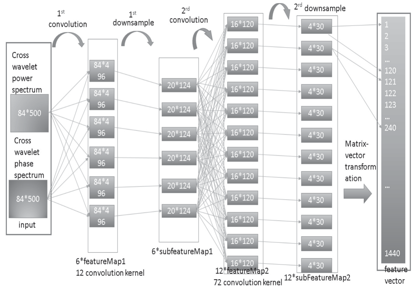
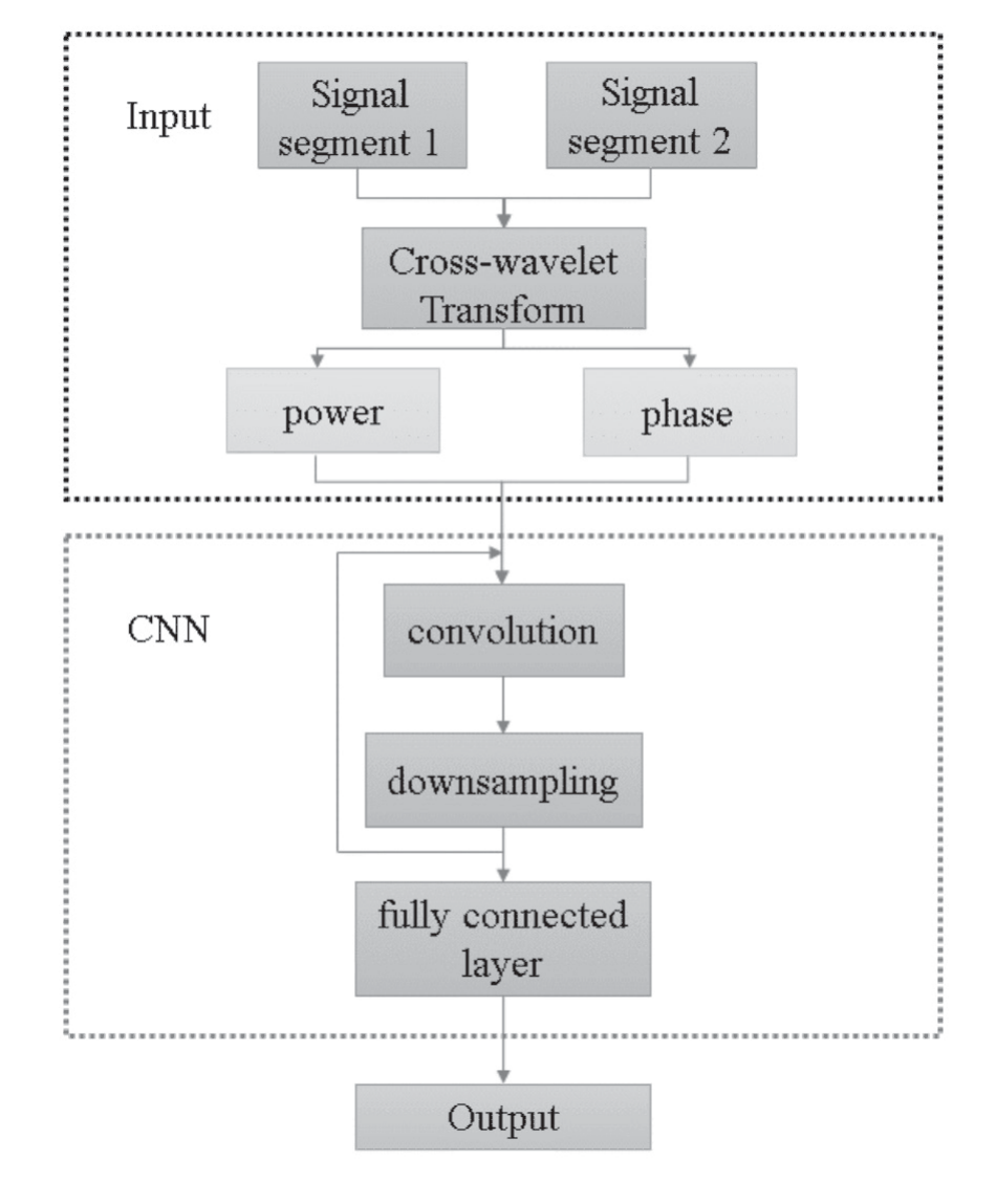
Fig. 8 is a schematic diagram of the proposed CNN model construction. Convolutional neural network (CNN) has the feature of weight sharing, which can deepen the number of neural network layers, reduce network parameters, and have a great improvement in feature extraction. It has accelerated development and breakthroughs in speech and visual recognition, natural language processing [49], microseismic wave shape data analysis and processing, and other fields. In fact, the microseismic wave shape also has translation invariance, which makes CNN suitable for the establishment of microseismic data classification models. In traffic tunnels like Micangshan Tunnel [50] and Bayu Tunnel [51], people have established an intelligent classification model of microseismic waves based on convolutional neural networks to classify microseismic signals, which has been well applied. Fig. 9 shows the general steps of the CNN method.
Noise Reduction
In the process of identification and classification, the signals are disturbed by noise. These disturbances include construction noise, instrument noise, mechanical noise, electrical noise, and other noises. They affect the work of microseismic monitoring seriously. So the reduction of noise becomes another key part of microseismic signal processing. The source parameters can be obtained to the maximum extent, and the accuracy and effectiveness of early warning can be further improved by reducing the noise [52, 53]. However, due to the complexity of the environment, this work is not so easy. It not only changes with time, but its frequency band also overlaps with that of the target signal.
Traditional methods of noise reduction cannot eliminate the noise completely. And it may cause distortion of the signal. On the one hand, the parameter settings of traditional noise reduction methods will affect the effect of noise reduction under the influence of different types of noise. On the other hand, traditional automatic extraction methods often need to adjust the algorithm parameters to achieve the best accuracy, which will further affect the accuracy of the signal source location. In the traffic tunnels, the different characteristics of microseismic monitoring signal noise will also have an impact on the noise reduction work. Firstly, the larger size of the traffic tunnel makes the number of signals collected huge, and thus the noise contained therein is more complex. Most importantly, the construction steps of the traffic tunnel are more complicated and tedious, which makes the noise signal more complex in time and space. Last but not least, a large number of different noises will affect the analysis of the tunnel structure during operation.
Many studies have been carried out to address these problems. Tselentis et al. [54] studied noise reduction based on the S-transform; L Smith et al. [55] studied noise reduction based on the short-time Fourier transform; Mousavi et al. [56] studied noise reduction based on the continuous wavelet transform; Wei et al. [57] studied noise reduction based on empirical modal decomposition; J Misztela et al. [58] studied noise reduction based on fuzzy mathematical noise reduction; W Jiang et al. [59] studied noise reduction based on singular spectrum analysis; Chen et al. [60] studied noise removal based on the sparse transform approach; Li et al. [61] studied noise removal based on the mathematical morphology approach; and K Huang et al. [62] studied noise removal based on non-local mean algorithm. In recent years, deep learning has emerged as a powerful machine learning technique that has brought great advances to signal and image processing [63]. Innovative ways based on deep learning for data interpolation and the reduction of noise have been proposed in image processing by residual-neural networks [64], generative adversarial networks, and convolutional autoencoders [65]. And some studies have shown that deep learning has been used to improve seismic noise reduction by learning better sparse representations [66-68] and has proven to be a powerful tool for learning features of seismic data [69-71].
Arrival Detection
Further analysis of the microseismic signal can be performed once the noise deduction and waveform identification are completed. Some key parameters of the earthquake source can be obtained from these parts, such as the time of occurrence, the location of the source, the corresponding intensity of the microseismic event, and the mechanism of the source. Early warnings of impending danger can be made based on that. And the detection of arrival time is the basis of this work. The microseismic signal can be regarded as a special kind of temporal data, and its temporality is reflected in its composition, which is P-band, S-band, and noise segment, in that order [71]. Arrival detection is much more difficult than signal identification because arrival detection of microseismic waves requries microscopic, ultra-long sequence processing with millisecond-level accuracy. There are also many research disciplines on arrival time detection.
(1) Long-Short-Term Window Ratio [72-74]. The ratio of Short-Term Average (STA) and Long-Term Average (LTA) is used to reflect changes in signal amplitude, frequency, etc. When a microseismic signal arrives, there is a sudden change in the STA/LTA value. A microseismic event can be determined when the ratio is greater than a certain set threshold. This method is the most common method used in commercial software for microseismic monitoring. It is computationally small and suitable for handling large batches of data. However, it is only robust to laboratory data with a very high signal-to-noise ratio and performs poorly on real engineering data filled with noise. In addition, the performance of the algorithm is also dependent on the choice of thresholds and requires human selection of appropriate thresholds.
(2) Akaike Information Criterion (AIC) [75]. The minimal point of the waveform curve, which can be calculated by AIC, is used as the arrival point of the P-wave. It is usually combined with other methods such as wavelet transform (wavelet-AIC) or Auto Regression (AR-AIC). The method associated with AIC performs well in actual seismic activity, but is prone to errors because local maxima and global maxima are not easy to separate [76]. And it is equally susceptible to background noise for microseismic data of low quality, i.e., data with a relatively small signal-to-noise ratio.
(3) Wavelet transform and frequency domain transform. Feature functions are set in other domains and combined with other methods such as K-Means, principal component analysis (PCA), and AIC for to-time picking [77-79].
(4) A data-driven method. The features are automatically extracted from a lot of labeled data with deep learning-based algorithms. For arrival detection, this part of the algorithm still has a relatively high accuracy [69, 80]. However, the length of microseismic monitoring signals is generally long, and the currently used deep learning architectures have problems dealing with such ultra-long sequence signals. The support for ultra-long sequences is yet to be completed. The imbalance problem will also lead to only one arrival point among thousands of sampling points, and model training will not converge.
Therefore, the long- and short-term memory network model can realize the comprehensive analysis of temporal information and complete the long-term preservation of information. However, it is difficult to pick up the accurate P-wave directly from the original data by using the long- and short-term memory network due to the characteristics of microseismic signal instability and a low signal-to-noise ratio. As can be seen above, both arrival detection and signal identification are affected by surrounding noise and static noise [81]. Although many noise reduction algorithms have been proposed by researchers [82], the use of these techniques results in the loss of information from the original data, causing the distortion of the signal. Therefore, the ideal way is to process the original data by the algorithm directly. In addition, many previous studies have been limited by the experimental data. Compared with the records in actual engineering, the experimental data are simple, lack of noise, and have few types of rupture signals due to the singularity of lithology. It is easy for the algorithm to achieve good results based on these data, while the errors caused in practical applications cannot meet the engineering needs.
Localization
Localization of microseismics is at the core of microseismic monitoring [83-85]. In this process, the microseismic monitoring system inferred the location of the rupture after processing the signals accordingly. Microseismic signals have similar mechanisms of source and signal characteristics as natural seismic signals, and therefore the localization methods are mostly cited from seismology [86]. In essence, it is a common inversion process in geophysics; that is, after analyzing the first arrival time of an event and the corresponding coordinate position, the corresponding spatial position is inversed The direct shear wave is easily disturbed by the subsequent wave in the tail of the longitudinal wave, so the longitudinal wave signal is mainly used to locate the source. In the actual work, the number of sensors is very large. Therefore, the process of inversion can be described as a process of solving super-stationary equations. The direct shear wave is easily disturbed by the subsequent wave in the tail of the longitudinal wave, so the main part used to locate the source is the longitudinal wave signal. The microseismic localization methods mainly include geometric localization methods, relative localization methods, spatial domain localization methods, linear localization methods, and nonlinear localization methods. According to the different localization principles, the localization methods can also be divided into two types; those based on three-axis sensors [87-90] and those based on the arrival-time difference theory [91-93].
The essence of the classical seismic localization method proposed by Geiger is to linearize the nonlinear system of equations and solve it using the least squares principle. The method involves partial derivatives and inverse matrix operations, which are computationally intensive [94]. With the development of computer technology, Geiger’s idea has been widely used. Also, various joint inversion methods [95], relative localization method [96], table-even time difference method [97], simplex method [98], double residual method [99], and Powll method [100] have contributed to the development of studies in earthquake source localization. These methods can be divided into 2 categories depending on the parameters involved in the solution [101]. One is the localization method, which uses a known wave velocity model to solve for the source time and location, also known as the classical method. The other is the joint method, which addresses the location, source time, and wave velocity model together. The classical method is most widely used in the seismic field and mining engineering. The inaccuracy of the wave velocity model is its disadvantage. Although there have been many studies on the wave velocity model, it is still a crucial problem affecting the stability and positioning accuracy of the location algorithm. The joint method addresses it better and improves localization accuracy to a large extent. However, the parameters of location, seismic time, and medium velocity in the joint method are not independent of each other, which means that the obtained solutions are not unique. This also poses difficulties in the selection of parameters. With the intercommunication and penetration of various disciplines, optimization methods from other fields have been used, such as genetic algorithms, particle swarm algorithms, simulated annealing methods, etc. [102-104]. The localization method has gradually developed from the mathematical model to the bionic model.
Traditional analysis of time series and machine learning choose features instead of the whole signal. The data may not be fully utilized due to subjective human factors. Deep-learning models can extract a large number of higher-order features automatically, thus making full use of waveform information. The data can be directly used as input to the neural network, avoiding the loss of information caused by manual selection. Deep learning is also well suited to handle the large amount of daily data. Many studies have also confirmed the potential and efficiency of deep learning over traditional methods in microseismic monitoring. However, the current network for microseismic signal identification still has disadvantages in certain parts.
(1) The simple network is limited in handling complex datasets containing a large number of atypical waveforms. Moreover, microseismic signals are often interrelated multi-channel signals, and processing multiple channels simultaneously consumes more resources, which is also not easily deployed on low-equipped machines in the field.
(2) More layers are usually added to the network to increase processing power. However, simply stacking layers may lead to network degradation [105] and gradient disappearance [106]. Moreover, each additional layer leads to a significant increase in the number of parameters and computational complexity. Some models even contain hundreds of thousands or even millions of parameters [107]. However, such complex models are not really needed to accomplish the task of waveform classification, and the deepening of the network would lead to redundant computations.
(3) Most of the microseismic signals currently processed using deep convolution save the signal as a picture and then use some open-source architectures of computer vision for processing. However, the features of the microseismic signal images are so different from those in the ImageNet dataset [108] that it is difficult to use the pre-trained weights of these architectures. And the scale of models of deep learning in the CV domain is very large, and the huge computational resource consumption makes the deployment and training of the models problematic.
Microseismic-Based Forecast and Early Warning
The prediction and early warning of rockburst refers to the early warning of rockburst by on-site monitoring data. The most important feature of microseismic monitoring in rockburst prediction and early warning is that the corresponding relationship between monitoring information and rock state is established by locating the instability area, and then the characteristics of signal changes during a rockburst are obtained. This information can be used as a precursor to rockbursts and can be used to predict their occurrence effectively. Most rock burst processes are characterized by microseismic information precursors [109]. Most microseismic events and their energy evolution in the process of an instantaneous rock burst have self-similarity and fractal characteristics of time, energy, and space [110-112]. This indicates that the location and burst level of a direct rock burst can be predicted by microseismic monitoring information in most cases. Its wide use in various underground engineering applications also shows that it is an effective tool to reveal rock blasting mechanisms and predict rock blasting [113-116].
According to the degree of fracture development, the three-dimensional spatial pattern of the excavation site, the distribution pattern of the stress field, and the distribution of the high in-situ stress area are determined, so as to predict the location and the degree and probability of the potential rock burst. The risk level of a rock burst can be automatically determined on the basis of the existing microseismic monitoring data, which can reduce the bias caused by the subjectivity of data analysts to a certain extent. This makes the identification result of the rock burst risk level in the traffic tunnel more objective and automatic. Based on the research results of earthquake - microseismic - acoustic emission and monitoring practices, the principle of early warning based on microseismic ground stress activity is proposed [117-119]. The flowchart for the rock burst warning can be obtained from Fig. 10.
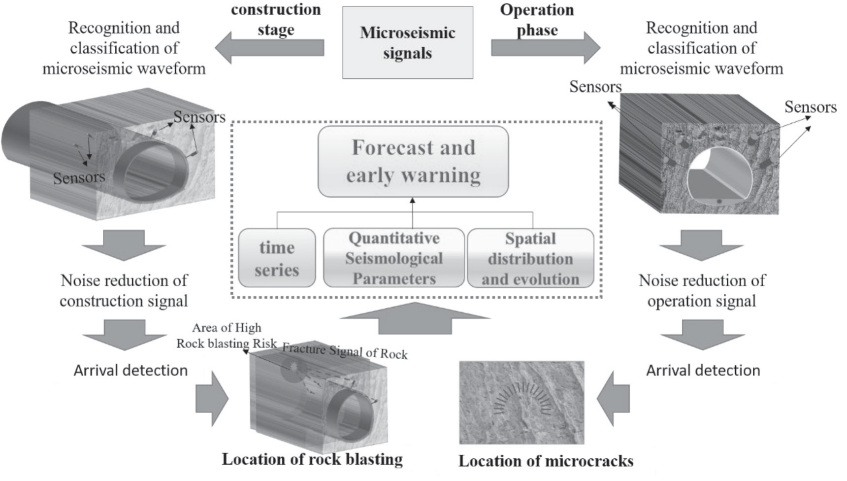
(1) Time series - Abnormal numbers or energy statistics of microseismic events.
In time-quantity statistics, the sudden and significant increase in the number and energy of microseismic events in a certain period of time indicates that rock activity is unusually frequent. At this time, attention should be paid to the activity intensity of the surrounding rock to prevent a rock burst. The energy level and frequency of microseismic events in a certain region and a certain monitoring period are consistently higher than the average or increase rapidly without an obvious alternating release process, which can be defined as an active period and requires warning. Based on this principle, many scholars have innovatively diversified time series methods to predict and warn of rock bursts. Wang et al. used the state variables reconstructed from multiple time series as inputs for the LSSVR model to predict and validate the future values of variables in rock burst monitoring. The results showed that this method can accurately predict monitoring variables, thereby predicting the occurrence of rock bursts [120]; Based on the frequency of microseismic activity and the time series curve of energy release, Liang et al. determined that the type of rock burst sequence in the tunnel is foreshock, main shock, and aftershock [34].
(2) Spatial distribution and evolution - Microseismic events induced by continuous rock rupture.
Microseismicity occurs continuously along a certain zone within a certain area of the tunnel excavation envelope and forms a regular distribution. At this time, the possible tectonic activation within the rock will cause an increase in stress accumulation in the surrounding rock and lead to rock-blasting disasters. Within a certain time interval, the energy level and concentration of microseismic events in this region increase rapidly, which can be defined as an active area; that is, an early warning is needed. Based on the spatiotemporal evolution laws of microseismic events, scholars have conducted some research on rock burst prediction and warning. Yu et al. studied the autocorrelation of microseismic event time distribution during rockburst evolution by establishing a fractal calculation method and defining the rock burst intensity based on the time fractal dimension [121]. Lai et al. used microseismic monitoring instruments and stress sensor monitoring systems to analyze the spatiotemporal distribution characteristics of microseismic events during tunnel excavation, providing a reference for rock burst warning in underground engineering in complex spatial environments [122].
(3) Quantitative seismological parameters.
The performance record of ground stress was fitted according to the change in specific index parameters. Firstly, the characteristics of the surrounding stress are summarized. Secondly, it summarizes its changing rules and puts forward the corresponding warning threshold. The above three parameters have strong guiding significance for rockburst prediction and early warning. However, multi-parameter early warning is prone to conflict in field applications, resulting in out-of-focus or generalization. When high-energy events occur, microseismic sensors around the tunnel can effectively monitor high-energy microseismic waves. When a high-energy microseismic event is detected within a certain period, positioning technology can analyze the location and type of rupture in a timely manner and, if necessary, predict the location of the rockburst to reduce the harm caused by the rockburst.
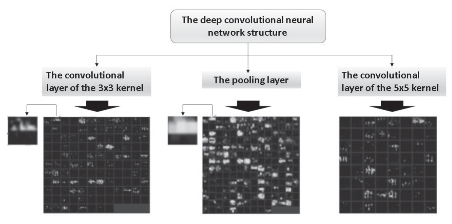
In the first stage, rockburst risk discrimination is mainly completed by researchers with highly specialized knowledge based on a comprehensive analysis of microseismic activity monitoring data. Affected by subjectivity, different personnel may come up with different discriminatory results. The energy index formed in the whole process of rockburst has great fluctuation and dispersion, and the warning accuracy cannot be guaranteed by observing its changing trend with the cumulative apparent volume manually. With the gradual quantification of rock blast risk discrimination indicators, it is possible to automatically discriminate the risk of a rock blast based on parameters. In the design of the burst risk level automatic discrimination system, the parameters and set values selected by users can be classified, sorted, and aggregated according to the current microseismic monitoring data, and the risk level of a rock burst can be finally determined. The process of rock burst warning by using the change trend of cumulative apparent volume and energy index can be considered a time series classification. Three classification stages (rockburst burst stage, rockburst mutation stage, and rockburst disaster stage) of the whole process of rockburst hazard source formation can be obtained by inputting the cumulative apparent volume and energy index. With the rapid development of computer technology, various types of deep learning methods have been applied to time series classification [123-125]. Fig. 11 shows a multi-layer DCNN model that has been proven to be applicable for signal classification and recognition. It means that rockburst warning has been improved with the help of these methods, too. Among them, the neural networks commonly used for TCS are Multi-Layer Perceptron, CNN, and Echo State Network, while CNN proved to be widely used for classification tasks.
Applications
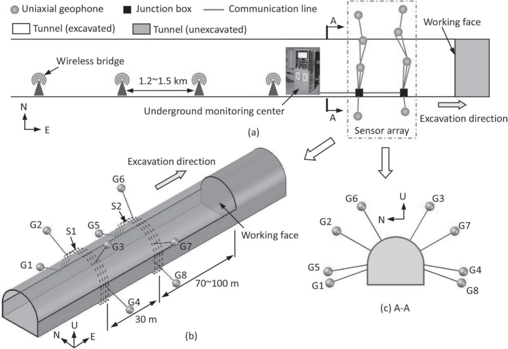
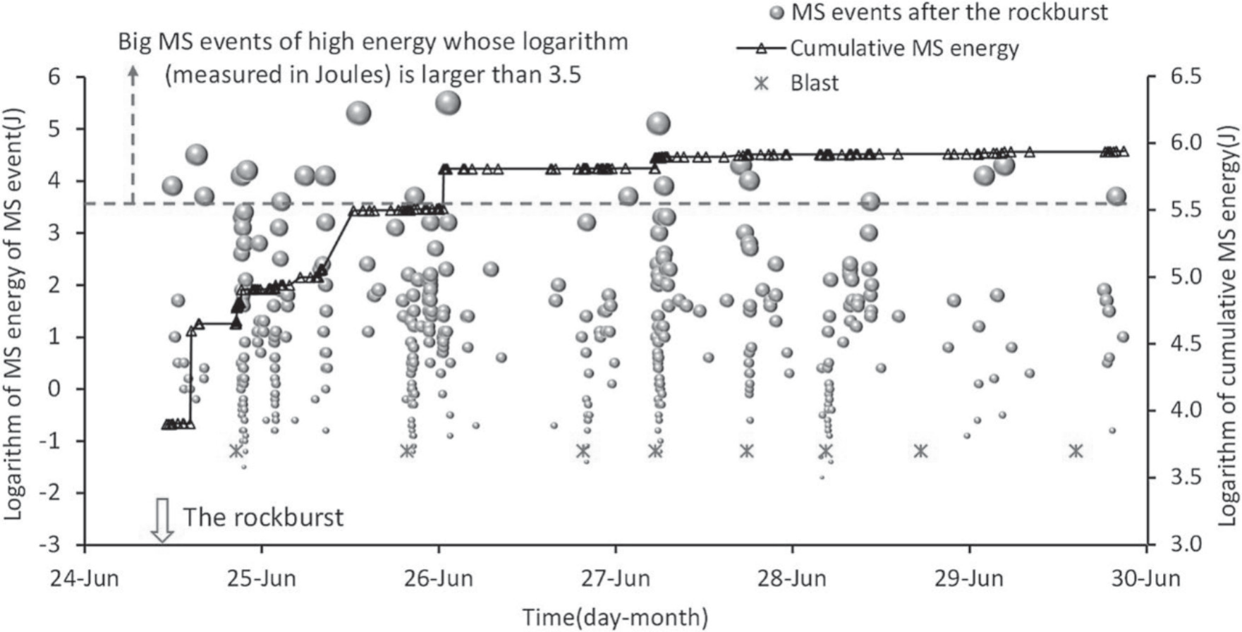
Since the establishment of the observation station in Germany in 1908, microseismic monitoring technology has been widely used in various kinds of tunnels. In China, it has also been widely used in the construction of the Bazhong-Shaanxi expressway, YeZhuping, Micang-mountain tunnel, and Bayu tunnel in recent years. For example, in the MCS tunnel, 221 microseismic events were recorded by the microseismic monitoring system. These microseismic events reflect a series of chain rupture processes of rock in two strong rock bursts and successfully predict the location of rock bursts many times. Fig. 12 shows the arrangement of microseismic monitoring sensors in a railway tunnel in southern China, and the details of microseismic activity detected after a single rock burst are shown in Fig. 13. It can be seen from Fig. 13 that each rock burst has a similar pattern; that is, the occurrence of each rock burst is always accompanied by a large number of microseismic activities.
In the BY tunnel, the microseismic events on both sides show uneven distribution characteristics. With the shift in rockburst location, the characteristic parameters of microseismic event density, microseismic release energy, and cumulative apparent volume show an obvious shift in the core area of the rockburst. The signal processing system includes a server, an analog-to-digital converter (ADC), a seismic processor (SP), and a power supply (PS), which can collect elastic waves and convert them into visual signals. The MS monitoring platform can receive visual signals from the wireless bridge and transmit them to the control center through the Internet. The control center analyzes the visual signal conveyed by the processing system and finally obtains the rockburst information from the surrounding rock. Most microseismic monitoring methods used in traffic tunnels have similar structures and mechanisms to those used in BY tunnels and the railway tunnels shown above. Through the application of microseismic monitoring technology in the above tunnel, it can be found that the disadvantage of microseismic monitoring is that it is easy to be affected by adverse conditions and the range of sensor layout. Therefore, by optimizing the placement of sensors, the mass spectral events can be located quickly and accurately, and real information about the rock microfracture source can finally be obtained.
Conclusion
In the situation of rock blasting frequently in traffic tunnels under high ground stress, this paper introduces microseismic monitoring. The six parts of microseismic monitoring, including signal acquisition, recognition and classification, noise reduction, arrival detection, localization, and prediction and warning, are described in detail. The differences between the application of microseismic monitoring in traffic tunnels and in mining tunnels are discussed in each process of microseismic monitoring. Although a lot of research has been done on both rock burst and microseismic monitoring under conditions of high ground stress, most of it has not been done in combination. At present, microseismic monitoring is mainly used in mining tunnels, hydraulic tunnels, slope engineering, and other fields. There is still a lot of work to be done to apply microseismic monitoring to the excavation of transportation tunnels. With the rapid development of world technology, traffic tunnels are moving towards larger cross-sections and longer distances. In addition, more diverse support methods during construction will make signal processing more difficult. These problems will bring trouble to the application of microseismic monitoring in traffic tunnels. Microseismic monitoring in traffic tunnels should pay more attention to the following aspects, such as improving the accuracy and credibility of microseismic images, improving instruments, enhancing the ability to deploy more sensors in tunnels to improve positioning accuracy, and deepening further research on data processing and positioning methods, including weak signal pickup. More importantly, the joint application of microseismic methods with other methods, the joint inversion of data, and the development of comprehensive data interpretation will better improve the monitoring accuracy of tunnels and the signal pickup rate. With the development of computers, artificial intelligence, and intelligent monitoring, reducing the harm of rock blasting will undoubtedly be effective.

