

Introduction
The escalating pace of urbanization coupled with current economic dynamics has magnified the challenge of urban air pollution, posing significant risks to public health, environmental integrity, and the broader paradigm of climate change [1, 2]. The intensification of anthropogenic activities, inclusive of industrial operations and the persistent reliance on fossil fuels, has led to an upsurge in the emission of key air pollutants such as Nitrogen Dioxides (NO2), Ozone (O3), Sulfur Dioxide (SO2), and Carbon Monoxide (CO) [3, 4]. These pollutants are pivotal in degrading air quality, with far-reaching implications for human health and environmental sustainability [5-7].
NO2 and SO2 have been identified as primary culprits in compromising the respiratory health of vulnerable populations, including children and the elderly [8, 9]. Short-term exposure to elevated levels of NO2 is associated with exacerbated asthma symptoms, increased incidence of emergency department visits, and heightened hospitalization rates [10, 11]. Prolonged exposure, on the other hand, is linked to a higher susceptibility to respiratory infections [12]. Moreover, the interaction of NO2 with other atmospheric constituents results in the formation of acid rain, whereas SO2 contributes to the generation of fine particulate matter [13, 14]. Both phenomena have deleterious effects on human health, damaging the respiratory system and exacerbating pre-existing health conditions.
O3 exposure is particularly concerning due to its capacity to induce a spectrum of adverse health outcomes, including inflammation, chronic pulmonary damage, and respiratory distress during physical activities [15, 16]. Vulnerable groups such as children, the elderly, outdoor enthusiasts, and individuals with pre-existing respiratory conditions like asthma are at heightened risk [17-19]. The detrimental health effects are compounded by the fact that O3 can interfere with lung function and provoke discomfort in the airways.
The impact of CO is equally alarming, with higher concentrations of this gas impairing the blood’s ability to transport oxygen effectively [20, 21]. This can have severe implications for vital organs, particularly the brain and heart, undermining their functionality and potentially leading to critical health outcomes [22-27]. In light of these findings, it is imperative to adopt comprehensive and integrated strategies aimed at mitigating air pollution. This involves transitioning towards cleaner energy sources, implementing stringent emission standards, and fostering public awareness about the health and environmental implications of air pollution [28]. By taking decisive action, it is possible to safeguard public health, preserve environmental quality, and contribute to the global effort to combat climate change [29].
In light of the recent findings that urban air pollutant concentrations exceed World Health Organization (WHO) thresholds, there is an urgent need to enhance air quality monitoring and forecasting, especially in rapidly developing nations like Vietnam [30, 31]. The integration of Smart City technologies, specifically the Internet of Things (IoT) and Information Communication Technology (ICT), presents a promising avenue for addressing these challenges [32, 33]. The Healthy Air project, implemented in Ho Chi Minh City (HCMC), utilizes a network of six wireless sensor-based air quality monitoring stations strategically located throughout the city [34-36]. This initiative underscores the critical role of advanced technologies in environmental management and public health protection.
The complexity of urban air quality management necessitates the development of sophisticated forecasting models that can accurately predict pollutant levels and inform public and policy responses. Traditional statistical methods such as moving averages and autoregressive models have been foundational in early attempts to model air quality [37, 38]. However, the intricate interplay between atmospheric conditions and pollutant concentrations demands more nuanced approaches that can adapt to dynamic environmental data and provide precise forecasts. Recent advancements in machine learning (ML) offer a robust framework for enhancing air quality prediction models [39-42]. ML algorithms, capable of processing large datasets and identifying complex patterns, are well-suited to the task of forecasting air pollution levels [43]. These models can leverage historical atmospheric data alongside real-time inputs from IoT-enabled monitoring stations to generate accurate predictions of future air quality [44-46]. Despite the potential of ML, the deployment of separate models for individual pollutants poses challenges in terms of efficiency, maintenance, and scalability [47-50].
To address these limitations, an integrated forecasting model that consolidates predictions for multiple pollutants could offer a more streamlined and effective approach. Such a model would not only reduce the operational complexity associated with maintaining multiple ML pipelines but also enhance the accuracy of air quality forecasts by considering the interdependencies between different pollutants. Furthermore, the limitations of traditional Vector Autoregression (VAR) models, particularly their reliance on stationary time series data, underscore the need for more adaptable forecasting methods [51, 52]. Advanced ML techniques, including deep learning and neural network architectures, could provide the necessary flexibility to handle non-stationary data and improve predictive performance [53].
The realm of air quality prediction has seen substantial advancements through the application of traditional machine learning techniques, which have proven adept at analyzing complex datasets and extracting critical features for model development [54, 55]. Among these, decision trees, support vector regression (SVR), artificial neural networks (ANN), and gradient boosting stand out for their efficacy in processing and interpreting environmental data [56-58]. Notable applications include the deployment of decision tree algorithms for categorizing air pollution indices and the integration of SVR with grey multivariable regression models to refine the accuracy of pollutant concentration forecasts [59-63]. Such approaches have showcased the potential of machine learning in uncovering non-linear relationships and latent patterns within air quality data, thereby illuminating the underlying dynamics of environmental factors.
However, the advent of deep learning has ushered in a new era of predictive modeling, characterized by its ability to construct intricate multi-layered neural networks. This advanced methodology has demonstrated superior performance in tackling the challenges posed by large datasets, high dimensionality, and complex nonlinear relationships inherent in air quality data [64-67]. Deep learning models, particularly convolutional neural networks (CNN) and graph convolutional networks (GCN), excel in distilling spatial correlations from data collected across multiple sites [68, 69]. Concurrently, long short-term memory networks (LSTM) and models employing self-attention mechanisms like Transformers and BERT have proven effective in capturing temporal dynamics and intricate spatio-temporal relationships. The main contributions of this study are: y This study introduces an advanced forecasting model,
EEMD+GRU+GCN_ATT, that integrates Ensemble
Empirical Mode Decomposition with Gated Recurrent
Units and GCN with attention, providing a significant
improvement in predicting ambient concentrations
of critical air pollutants (PM2.5, NO2, SO2) with high
accuracy and reliability across various statistical
metrics (MAE, MSE, MAPE, R2). y The research highlights the limitations of conventional
GCN models in air quality forecasting and
demonstrates the enhanced performance of models that
incorporate advanced neural network architectures and
decomposition techniques, addressing the complex
spatio-temporal dependencies in environmental data
by adding an attention mechanism. y The study contributes to the field of environmental
monitoring and policymaking by offering a
robust tool for air quality forecasting, which can
significantly benefit public health and ecological
protection through more informed decision-making
and policy development.
Materials and Methods
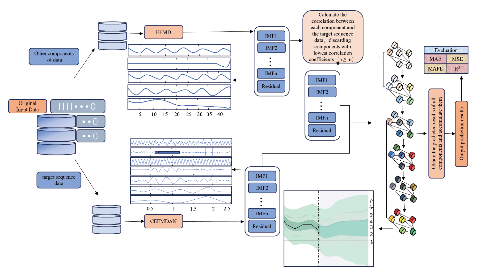
Before describing the proposed model used for time series data prediction, we will briefly discuss the related fundamental theories behind this model construction, namely, the EEMD, the CEEMDAN, and the principles and applications of the attention. Fig. 1 shows the complete implementation of the model used in this study.
GCN Model
Implementing a Graph Convolutional Network (GCN) with an attention mechanism for climate prediction involves a series of steps. The process combines the relational inductive biases inherent in GCNs with the focusing ability of attention mechanisms to prioritize the most relevant features and interactions for predictive tasks. The steps of the mode are:
Define the Problem:
Climate prediction variable collection (e.g., temperature, precipitation, extreme weather events).
Determine the scale of the dataset (local, regional, global).
Data Collection:
Gather historical climate data (temperature, humidity, precipitation, etc.) from various sources like weather stations, satellite images, or climate models.
Include relevant auxiliary data that can impact climate patterns (e.g., oceanic conditions, solar cycles, anthropogenic factors).
Data Preprocessing:
Clean the data to handle missing values, anomalies, or outliers.
Normalize or standardize the features to ensure that the scale of the data does not bias the attention mechanism.
Graph Construction:
Create a graph where nodes represent different geographic locations or climate variables, and edges represent the connections or correlations between these nodes (spatial, temporal, or feature-based relationships).
Feature Engineering:
Select or engineer features for each node based on the data and problem at hand, including temporal dynamics.
Graph Convolutional Network Design:
Design the GCN architecture, specifying the number of layers and the dimensionality of the node representations.
Incorporate attention mechanisms within the GCN layers to weigh the influence of neighboring nodes dynamically.
Model Training:
Split the dataset into training, validation, and testing sets.
Train the GCN with an attention mechanism using the training set, applying backpropagation and an appropriate optimizer.
Regularly evaluate the model on the validation set and use early stopping or other regularization techniques to prevent overfitting.
Hyperparameter Tuning:
Experiment with different hyperparameters such as learning rate, number of GCN layers, attention heads, and hidden unit sizes to optimize model performance.
Model Evaluation:
Assess the model’s performance on the test set using metrics relevant to climate prediction, such as RMSE for continuous outputs or accuracy for categorical events.
Interpretation and Analysis:
Interpret the model’s attention weights to understand the influence of different features or locations on the prediction.
Analyze the model’s predictions in the context of known climate patterns and dynamics.
Model Deployment:
Integrate the model into a decision-making framework for climate adaptation strategies or further scientific research.
Implement a user interface for stakeholders to access and utilize the climate predictions.
Model Updating:
Regularly update the model with new data to refine predictions and capture evolving climate patterns.
Re-train or fine-tune the model as necessary to maintain its accuracy over time.
This high-level overview provides a framework for utilizing GCN with an attention mechanism for climate prediction. Implementing each step would require detailed technical planning, execution, and a deep understanding of both machine learning techniques and climate science.
Ensemble Empirical Mode Decomposition (EEMD)
Shih-Lin Lin [70] proposed the Ensemble Empirical Mode Decomposition (EEMD) method, which emerges as a virtuoso in the world of signal representation. This exquisite technique unveils the soul of unpredictable and not linear oscillations, crafting a prelude of transformation from raw data.
EEMD is an enhanced technique based on Empirical Mode Decomposition (EMD). EEMD adds Gaussian white residue to the original data for EMD decomposition, which successfully solves the issue of mode mixing and last-point effects in traditional EMD. The algorithm framework of EEMD is shown in Algorithm 1. The calculation process of the EEMD algorithm is as follows:
1) Add Gaussian white noise to the original data to generate a new data set, as shown in formula (1).
Where
2) Decompose the new sequence data with added white noise,
Here, is the j-th IMF obtained after adding white noise for the i-th time, while represents the residual component obtained after adding white noise, which identify the mean trend of the signal. n shows the number of IMF components.
3) Repeat the above steps m times, adding different white noise each time, to obtain n decomposition results of m sequences:
4) Utilizing the characteristic of Gaussian white noise having a mean of zero, take the average of the individual IMF value and the residual component obtained from the previous steps, and sum them up to obtain the final output, as shown in formula (4):
Complete Ensemble Empirical Mode
Decomposition with Adaptive Noise (CEEMDAN):
For addressing nonlinear nonstationary data, Quinn et al. [71] presented an adaptive signal processing technique called EMD. EMD doesn’t necessitate any data constraints and can break down complicated unpredictable patterns while keeping the data’s time scale. Modal mixing is a challenge that EMD frequently faces in practical applications, though [70] therefore offers EEMD based on EMD. Based on the assumption that the average value of the white noise is zero, EEMD breaks down the data by continually adding different white noise to the original values. The modal mixing problem can be significantly improved in this way, but there are drawbacks, including a significant upper reconstruction error and a lengthy calculation time. The EEMD-based CEEMDAN is therefore suggested as a solution to the aforementioned issues. By incorporating adaptive white noise, CEEMDAN not only successfully addresses the issue of modal mixing, but also eliminates the reconstruction error and lowers computation costs. CEEMDAN is hence better able to handle non-smooth and non-linear data.
The CEEMDAN algorithm, as shown in Algorithm 2, is also an improved method based on EMD. It overcomes the mode mixing problem in EMD. Unlike EEMD, CEEMDAN doesn’t directly sum up Gaussian white noise to the original signal but includes auxiliary noise to the mode components obtained after EMD decomposition. At the same time, the overall average calculation begins after obtaining the first mode component and continues until obtaining the final mode component. This process is then repeated for the residual component. The calculation method of the CEEMDAN algorithm is as follows:
Where
2) Perform EMD decomposition on each new signal with added Gaussian white noise to obtain the first Intrinsic Mode Function and the residual component, as shown in formulas (6) and (7):
Here, E represents the EEMD decomposition operation.
, and obtain the , as shown in formula (8):
Data Sets and Evaluation Metrics:
Study Area
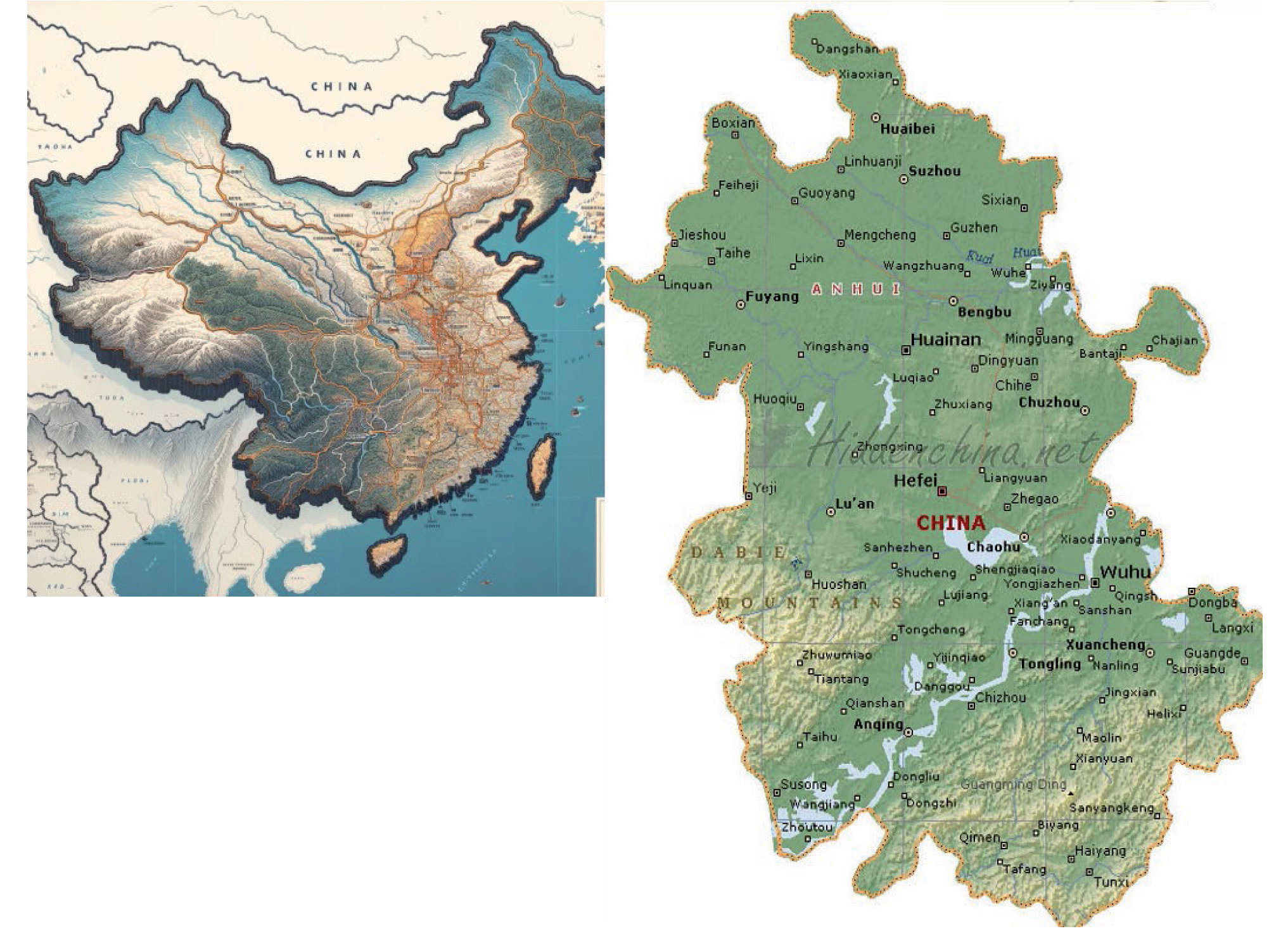
Anhui are provinces in China with diverse geographical features and unique characteristics. Anhui Province, located in eastern China, experiences a diverse climate ranging from humid subtropical in the south to humid continental in the north, with distinct seasonal variations characterized by hot, humid summers and cool, somewhat dry winters. This climatic variation supports a variety of agricultural activities, making Anhui known for its tea production, particularly Huangshan Maofeng and Keemun tea. The province’s economy is also bolstered by its growing industries in machinery, electronics, chemicals, and textiles, contributing to its status as a significant player in China’s economic landscape. However, rapid industrialization and urbanization have led to environmental challenges, including air pollution. The reliance on coal for energy and the density of vehicular traffic contribute to the emissions of particulate matter (PM2.5 and PM10), nitrogen dioxide (NO2), and sulfur dioxide (SO2), impacting public health and necessitating concerted efforts in air quality management and sustainable development practices to mitigate pollution levels. The study area, its location in China, and the monitoring stations of the Province are to be used and shown in Fig. 2.
Data Sets
The requirements for ambient air quality and the effects of various contaminants on flora, fauna, and the environment serve as the foundation for the air pollution index. A single conceptual index value is used to represent the concentration of all consistently measured air pollutants. This study takes 1-year air pollutant data (From 01-2021 to 12-2021) for performing the algorithm testing and verification. We separated all datasets into 8:1:1 training, validation, and testing sets.
Evaluation Metrics
In this study, four evaluation metrics were selected to assess the effectiveness of the offered models’ predictions, namely: Mean Absolute Error (MAE), Mean Square Error (MSE), Mean Absolute Percentage Error (MAPE), and R2 (R Squared). Their formulas are as follows:
yi signifies the actual value of the time series sample, denotes the model’s predicted value, n means the number of testing samples, and i represents the sequence number of the testing sample in the above formulae.
Results
A. Particulate Matter:
Table 1 appears to present a comparative analysis of different deep learning models based on their performance in predicting air quality or a similar metric. Each row represents a model and the columns show different statistical metrics used to assess the model’s predictive performance:
GCN (Graph Convolutional Network): This model has a balanced performance with respect to the evaluation metrics. It has moderate values of Root Mean Square Error (RMSE), Mean Absolute Error (MAE), Mean Square Error (MSE), Mean Absolute Percentage Error (MAPE), and a coefficient of determination (R2) of approximately 0.556. The relatively lower RMSE and MAE suggest that the GCN model has a decent fit to the data with modest prediction errors.
EMD+GCN (Empirical Mode Decomposition + Graph Convolutional Network): Incorporating EMD with GCN has improved the model’s performance slightly compared to the standalone GCN model. This is evidenced by lower RMSE, MAE, MSE, and MAPE, and a higher R2 value (0.577), indicating better prediction accuracy and model fit.
EEMD+GRU+GCN (Ensemble Empirical Mode Decomposition + Gated Recurrent Unit + Graph Convolutional Network): This model shows a significant increase in error metrics (RMSE, MAE, MSE) and a higher MAPE compared to the first two models, indicating less accuracy in prediction. The R2 value is also lower (0.511), suggesting that the model’s predictions are not as closely aligned with the actual values.
GCN_ATT (Graph Convolutional Network with Attention mechanism): This model has the highest errors (RMSE, MAE, MSE) and a relatively high MAPE, coupled with the lowest R2 value (0.439), indicating that the model performs the worst among the four in predicting the target variable.
RMSE (Root Mean Square Error): Lower values are better.
GCN: 14.77
EMD+GCN: 14.41 (Best)
EEMD+GRU+xGCN: 22.06
GCN_ATT: 23.63 (Worst)
The EMD+GCN model has the lowest RMSE, indicating that on average, its predictions are closer to the actual values. The GCN_ATT model has the highest RMSE, suggesting its predictions are the least accurate on average.
MAE (Mean Absolute Error): Lower values are better.
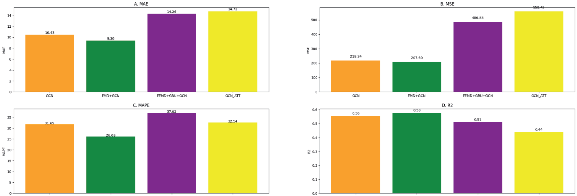
GCN: 10.43
EMD+GCN: 9.36 (Best)
EEMD+GRU+GCN: 14.26
GCN_ATT: 14.72 (Worst)
The EMD+GCN model has the lowest MAE, indicating it has the smallest average error in its predictions. The GCN_ATT has the highest MAE, meaning its average prediction error is the largest.
MSE (Mean Square Error): Lower values are better.
GCN: 218.34
EMD+GCN: 207.60 (Best)
EEMD+GRU+GCN: 486.83
GCN_ATT: 558.42 (Worst)
Again, the EMD+GCN model outperforms the others with the lowest MSE, implying its predictions have the least variance from the actual values. The GCN_ATT model’s predictions vary the most from the actual values, as indicated by its highest MSE.
MAPE (Mean Absolute Percentage Error): Lower values are better.
GCN: 31.65
EMD+GCN: 26.08 (Best)
EEMD+GRU+GCN: 37.02
GCN_ATT: 32.54
The EMD+GCN model has the lowest MAPE, meaning its prediction errors are smaller when compared as a percentage of the actual values. The EEMD+GRU+GCN has the highest MAPE, indicating less accuracy relative to the actual value scale.
R2 (Coefficient of Determination): Higher values are better, with 1 being a perfect prediction.
GCN: 0.556
EMD+GCN: 0.577 (Best)
EEMD+GRU+GCN: 0.511
GCN_ATT: 0.439 (Worst)
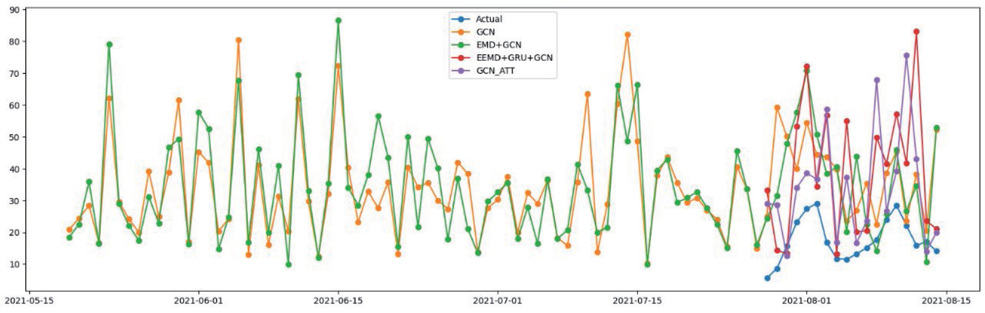
The EMD+GCN model again has the highest R2 score, indicating that it can explain the variation in the target variable better than the other models. The GCN_ ATT model has the lowest R2, suggesting that it has the least explanatory power regarding the variance in the data. EMD+GCN model consistently performs the best across all metrics, indicating it is the most accurate and reliable for predicting the target variable in this scenario. Conversely, the GCN_ATT model consistently scores the worst by these metrics, suggesting it might be the least suitable model for this particular prediction task. The addition of the EMD process appears to enhance the predictive power of the GCN, while the attention mechanism in GCN_ATT does not confer the same benefit. Fig. 3 shows the visual representation of models while Fig. 4 shows the time series difference in prediction from time to time.
Table 1.
Comparison of different models for Particulate Matter
B. NO2:
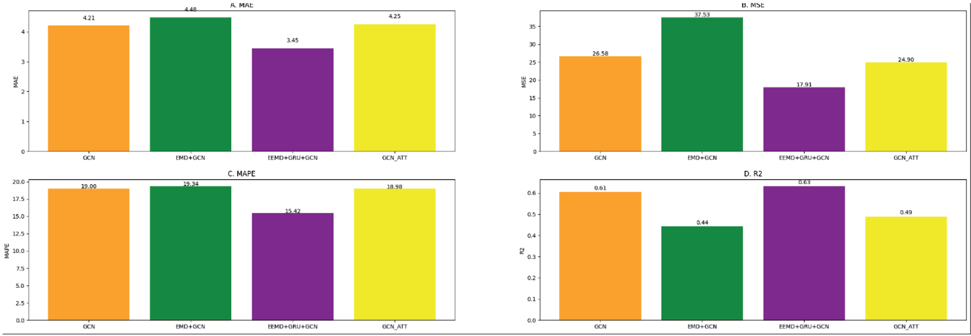
Fig. 5 shows the comparing performance of four different predictive models across four metrics. The EEMD+GRU+GCN model has the highest R^2 value, suggesting it best captures the variance in NO2 levels.
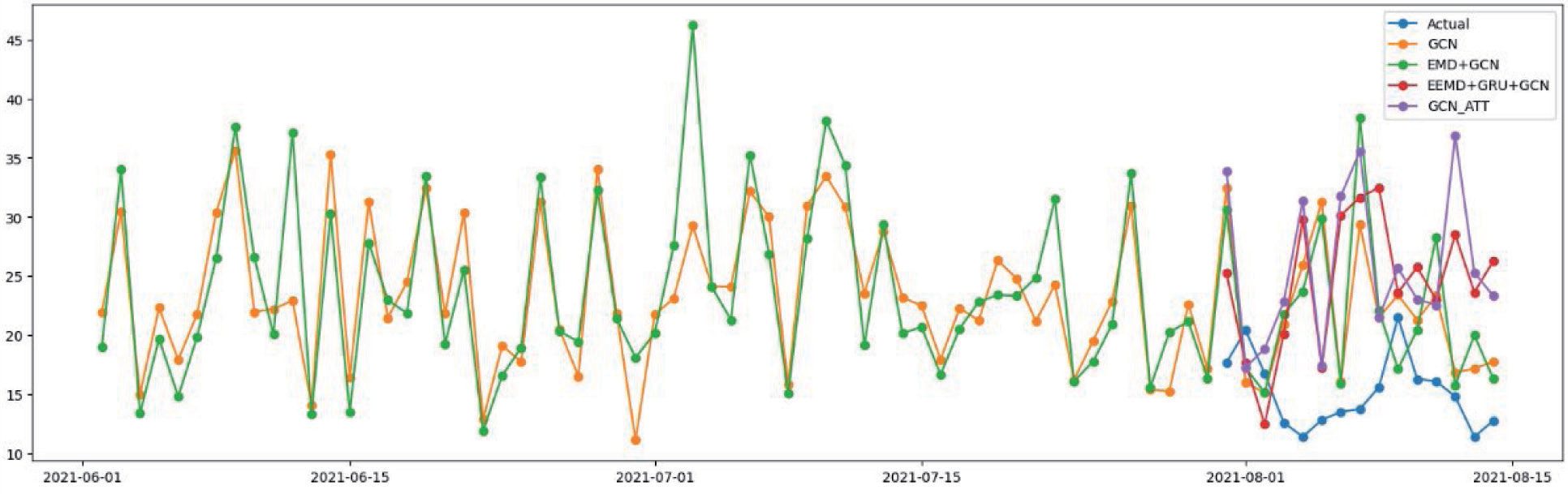
Across all metrics, the EEMD+GRU+GCN model consistently shows superior performance in predicting NO2 levels, implying it can handle the complexity of the data well. On the other hand, the EMD+GCN model seems to underperform, especially in terms of MSE, where it has the highest value indicating a poorer fit to the data compared to the other models. The GCN and GCN_ATT models show moderate performance across all metrics. Fig. 6 shows the time-to-time variation of the pollutants.
C. SO2:
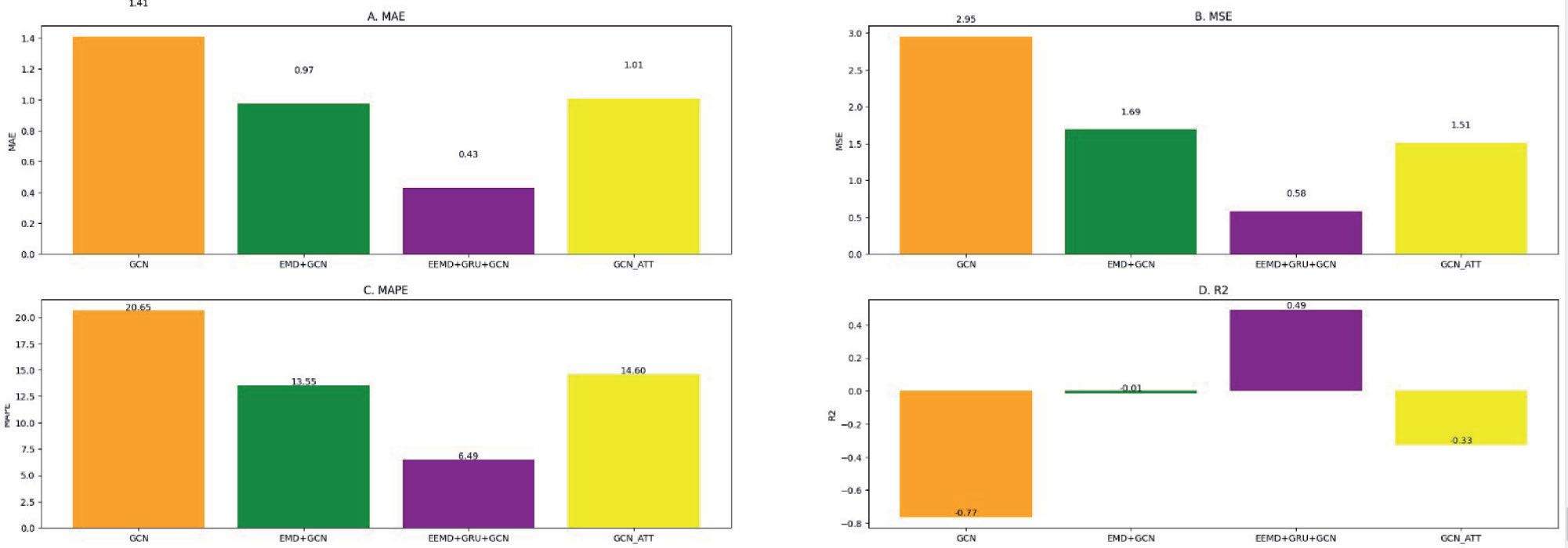
Fig. 7 compares the performance of four predictive models using four different evaluation metrics for the prediction of SO2 (sulfur dioxide) levels. An R^2 value, as seen with the GCN and GCN_ATT, indicates that the model fits the data worse than a horizontal line (i.e., a simple average). On the other hand, the EEMD+GRU+GCN model has an R^2 close to 0, suggesting that it’s barely capturing the variance in the SO2 levels, but it’s still the best among the compared models.
The EEMD+GRU+GCN model significantly outperforms the other three models across all metrics for SO2 prediction. It consistently demonstrates the lowest errors and the highest (or least negative) R^2 value, indicating its superior predictive accuracy and ability to capture the variance in the SO2 level data compared to the other models.
While the findings of this study offer promising directions for air quality prediction using deep learning models, several limitations must be acknowledged:
Model Generalization: The study’s models were tested and validated on specific datasets, which may not represent the full spectrum of air quality conditions globally. Generalizing these results to other regions or pollutants without additional validation could lead to inaccuracies.
Data Quality and Availability: The performance of the predictive models is heavily dependent on the quality and granularity of the input data. Gaps in data, inaccuracies in measurement, or lack of data diversity can negatively impact model performance.
Complexity of Atmospheric Phenomena: The models may not fully account for the complex chemical and physical processes that govern atmospheric pollution. Simplifications necessary for computational modeling might omit critical dynamics of pollutant dispersion and transformation.
Spatial and Temporal Dynamics: While the EEMD+GRU+GCN model captures spatio-temporal dependencies effectively, there may still be room for improvement, especially in capturing the long-range transport of pollutants or sudden changes due to extreme events.
Computational Demands: Advanced models like EEMD+GRU+GCN can be computationally intensive, which might limit their practical deployment, especially in real-time or resource-constrained scenarios.
Interpretable AI: Deep learning models often operate as ‘black boxes,’ providing little insight into how predictions are derived. This lack of transparency can be a barrier for trust and understanding in environmental management contexts.
Impact of External Factors: The models might not fully account for external factors such as policy changes, economic activities, or unexpected events like wildfires and industrial accidents, which can significantly affect air quality.
Algorithmic Bias and Overfitting: There is a risk of overfitting particular patterns present in the training data, which could lead to poor performance on unseen data. Moreover, algorithmic biases may arise from non-representative training datasets.
Dynamic Feature Selection: The study did not explore the impact of dynamic feature selection, which could potentially improve model performance by adapting the input features over time as more data becomes available.
Evaluation Metrics: The reliance on standard metrics like MAE, MSE, MAPE, and R2 provides a conventional assessment of model performance but may not fully capture the practical utility of the predictions in real-world decision-making scenarios.
These limitations highlight the need for ongoing research to refine predictive models further, to ensure robust and reliable air quality forecasting across diverse environmental conditions and to support informed decision-making for public health and environmental policy.
Conclusions
In conclusion, the comparative analysis of various advanced deep learning models for the prediction of key air pollutants—PM2.5, NO2, and SO2—has yielded significant insights. The study demonstrates the substantial potential of combining ensemble empirical mode decomposition with Gated Recurrent Units and Graph Convolutional Networks (EEMD+GRU+GCN) in accurately forecasting air quality indices. This model has consistently outperformed its counterparts across a suite of statistical measures, evidencing lower mean errors and stronger correlations with the observed data. Conversely, traditional GCN models and those augmented with attention mechanisms (GCN_ATT) have been shown to be less effective, particularly evidenced by negative R2 values in certain cases, suggesting a poor fit for the data at hand. These findings suggest that the complexity of air quality data, with its inherent spatial and temporal correlations, is more effectively captured by models that can adapt and learn from a multitude of data features and sequences, as is the case with the EEMD+GRU+GCN model. The results underline the importance of model selection in environmental data science and the need for continuous refinement of predictive algorithms. The superior performance of the EEMD+GRU+GCN model opens avenues for its application in real-world environmental monitoring systems, which can aid policymakers and health professionals in mitigating the impacts of air pollution. This research thus contributes to the growing body of knowledge in environmental informatics and underscores the pivotal role of machine learning in advancing public health and ecological conservation efforts.
Future work in the realm of air quality prediction using deep learning should focus on addressing the limitations identified in this study. Efforts could be made to enhance model generalization by testing and validating the models across diverse geographic locations and environmental conditions. Incorporating more comprehensive datasets, possibly enriched with data from satellite observations and more granular ground-level monitoring, will improve the robustness and accuracy of the predictions. Furthermore, the integration of explainable AI techniques can provide transparency into the decision-making process of these models, increasing their trustworthiness and utility for policymakers.

