


Introduction
Wastewater management and reuse are integral to water resources management [1]. Efficient wastewater management includes collection, treatment, discharge into nearby streams, and/or reuse [2]. All these phases of wastewater management require proper accounting for the quantities and quality of the wastewater. When wastewater is poorly managed, however, it may lead to environmental degradation [2]. Typical contaminants found in urban wastewater that can degrade surface water include nutrients such as phosphates, nitrates, nitrites, and ammonia [3]. These nutrients cause eutrophication of surface water bodies, among other environmental problems [3, 4]. Several reports of surface water pollution arise from discharging inefficiently managed wastewater. Liu et al. [5] stated that the highest surface water pollution rate in the world can be found in Central, Southeast, and East Asia (including China). The authors attributed surface water pollution to increased urban wastewater discharge, which, in turn, is directly linked to increased population growth and industrial activities. In Ghana, it was found that illegal mining activities heavily polluted the Pra River and consequently drained the acid mine into the river [6]. The study on the Pra River is further complicated by reports that people still use the polluted water for domestic purposes due to a lack of alternative clean water sources. Similar reports from Addis Ababa in Ethiopia show that 90% of the effluents from industrial and agricultural activities are released into nearby surface water bodies without proper treatment, leading to ecosystem damage and a decline in the quality of the impacted rivers [7]. When wastewater is managed correctly, however, the benefits are invaluable. For example, reusing treated wastewater can lead directly to conserving groundwater and other freshwater resources [1]. Studies also show that wastewater reuse can be engaged to combat the problems of water stress and scarcity [8]. Treated wastewater can be used as an alternative to freshwater for activities such as irrigation, landscaping, navigation, recreation, and other non-human skin contact purposes [9], thus decreasing pressure on freshwater sources.
However, converting wastewater into a valuable resource and an alternative to freshwater requires collecting wastewater generation data. Such data is necessary to design the required collection, treatment, storage, and transmission infrastructure. One method that has found useful application for analyzing wastewater data is the artificial neural network (ANN). Several studies have applied ANN to achieve wastewater quality and treatment efficiency. For example, Mohammad et al. [10] utilized ANN to model the removal of chlorophenols from wastewater via reverse osmosis. Findings from that study revealed that the neural network was used to accurately estimate chlorophenol rejection in the system. Also, ANN was adopted by Hamada [11] to predict the performance of the wastewater treatment plant in Gaza. In this study, the ANN model proved to be better than the multiple linear regression (MLR) model for predicting water quality parameters, which was comparable to another study carried out by Bekkari and Zeddouri [12], who utilized ANN to predict the performance of the Touggourt Wastewater Treatment Plant in Algeria regarding COD. Several other studies utilizing the ANN modeling approach in wastewater treatment have indicated different benefits, such as higher efficiency and accuracy [13, 14]. However, few studies have applied ANN to wastewater volume prediction for management purposes. Therefore, the current study aims to bridge this gap by using an artificial neural network (ANN) to account for current and future volumes of wastewater that will be received at a wastewater treatment facility. The study can also be extrapolated to the problem of inadequate capacity of a wastewater treatment plant (WWTP) infrastructure. Due to rapid population growth and the attendant increase in wastewater volumes, existing WWTPs often become inadequate. Without sufficient funds or physical space to expand the infrastructure, predicting expected wastewater volumes for management purposes becomes a cheaper alternative.
Materials and Methods
Study Area
The study location is the campus of a private institution of higher learning in the Ota community, Ogun State, Nigeria. The campus was selected for the study because it provides a relaxed environment to study diverse behaviors and activities that influence wastewater generation patterns. Additionally, the campus environment facilitated more comprehensive data collection because of the relative safety of the campus for personnel and research equipment. Typically, industry managers do not permit researchers to collect wastewater data because of the fear of documented evidence of their pollution activities and the attendant regulatory penalties. Nevertheless, the procedure laid out in this study can be adapted to study urban or industrial wastewater volume prediction. The study area is located approximately 16 km from the Lagos border and 81 km from the Ogun state capital, Abeokuta. The university community is rapidly growing with an annual enrollment of about 8079 students [1]. The community relies exclusively on groundwater, thus putting immense pressure on groundwater resources.
Previous studies on the same campus showed an increase in wastewater generation from 874,081 l/day in 2013 to 1,512,000 l/day in 2015 [8, 15], with the treated effluent discharged into the nearby Atuwara River. Due to the overloading of the WWTP, the treatment efficiency became compromised, leading to reports of fecal matter in the river body [14]. This problem, which was caused by the rapid growth in the student population, constitutes a significant threat to public health [15]. These problems led the institution’s managers to consider alternatives that address treatment efficiency and the possibility of reuse.
Data Collection
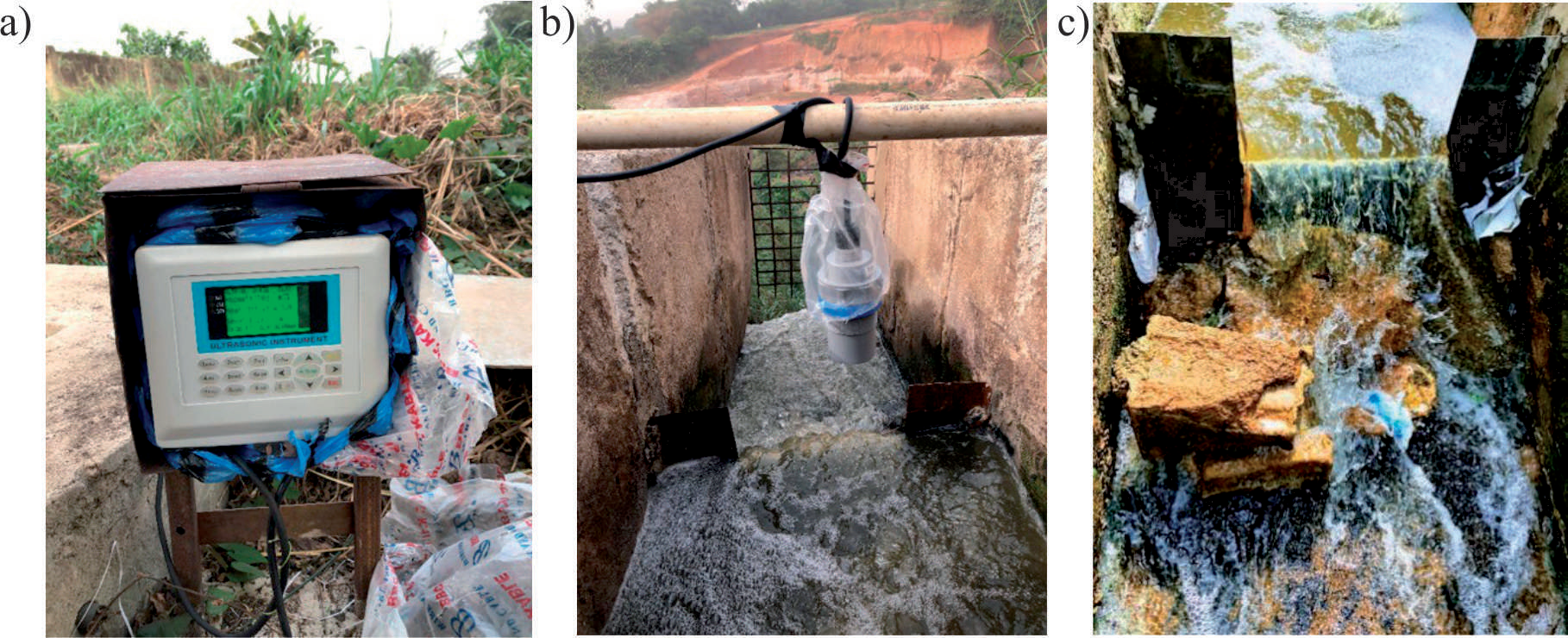
Wastewater generation data was collected and automatically recorded on an hourly basis for 24 hours over a total period of 81 days (23rd December 2019 to 12th March 2020) using an Ultrasonic Open Channel Flowmeter (model number: HOH-L-CF (M191022001)). This period of 81 days captured both the base flow and maximum flow (from the holiday season when students are away from campus and the season when the university is in session, respectively). Due to time constraints for the field investigation, an 81-day period that strategically coincides with the end of the dry and the start of the wet seasons was chosen for the wastewater volume data collection. This approach aims to ensure that the results accurately reflect the seasonal variations and their impact on water use and wastewater generated. The 81-day period also coincides with the peak population when the campus hosts hundreds of thousands of visitors for an annual event and the holiday season, which typically has the lowest population levels. The ultrasonic open channel flow meter is used to determine water levels in a channel by transmitting ultrasonic (sound) pulses from a sensor to the surface of the flow stream, and it measures the time (t) and velocity of the echo (c) that returns to the sensor. The equipment also stores data for subsequent retrieval. The ultrasonic flowmeter consists of two major components, a probe and a host, as depicted in Fig. 1(a-c). A temperature sensor is integrated into the probe to compensate for changes in air temperature, thus enhancing maximum accuracy.
For this study, a rectangular weir was fabricated to regulate the water flow. The probe was installed on the upstream side of the weir at a distance of 0.5 m from the weir and protected from direct sunlight and strong winds. The weir specifications were uploaded into the host using the weir type number in the manual. This initial calibration enabled the flowmeter to utilize pre-programmed discharge equations to generate the flow rate. The instantaneous flow rate and temperature were recorded and stored on the host hourly for subsequent retrieval. Daily flow rates were also recorded.
Artificial Neural Network
Artificial Neural Network (ANN) is a machine learning technique that emulates the operation of the human brain. It has been applied to various modeling problems [13, 14]. ANN uses processing units known as neurons. The operation of the neural network can be generalized using the following Equations.
Each link in the ANN model has an allocated weight, wkj. This weight is multiplied by its input, xj, and added to an external bias, bk. yk represents the output signal. φ is an activation function that is used to control the amplitude range of yk. In this research, the activation function to be used is the sigmoid function, and it is expressed as follows:
Equation (2) is the most frequently used activation function. ANNs can be set up using different model types. The model type used for this research is the multilayer perceptron (MLP). Depending on the architecture required, it can have one or more hidden layers, a single input layer, and a single output layer. For the essential operation of this model, the input data is supplied to the input layer, and the hidden layer collects this input and generates the output. The user at the output layer then receives this output. Neurons between layers are interconnected, and this is what makes it possible to obtain an output. MLP is also known as a feed-forward neural network. In the input layer, the neuron output is represented by Equation (3):
Where P represents the number of neurons in the input layer. Furthermore, the output is fed into a hidden neuron in the hidden layer, and the output of this layer is represented by Equation (4):
Fig. 1.
Picture of the Ultrasonic Open Channel Flowmeter in operation: a) host, b) probe, and c) weir.
Where φ is the activation function, Kh and P are the number of the hth hidden layer neurons and their inputs, respectively. Nh is the number of hidden layers.
The result at the output layer is obtained by adding the outputs generated at the hidden layer; this is expressed as follows:
Where T is the total number of neurons in the output layer. wkh,t is the weight of the connecting link of the hidden layer.
This study used the ANN toolbox in MATLAB to develop a model to predict the volume of wastewater generated within the university. A heuristic approach was adopted to obtain the best parameters and training algorithm. The data set for the development of the model was collected by installing a flow meter at the discharge point of the Covenant University wastewater treatment facility for 81 days. This data was divided into training, testing, and external testing datasets. Fifty data samples were used to train, and twenty were used for testing. Testing can be subdivided into validation and testing, depending on the training algorithm used by the model. Eleven data samples were separated from the rest of the data set and used to perform an external test after the model had been developed (created, trained, and validated).
Two models were developed from two training algorithms (Bayesian Regularization and Levenberg-Marquardt). The output results were compared to determine the best-performing algorithm. The data fed into the neural network fitting tool had nine inputs and one output. The output variable was the generated wastewater volume in cubic meters. The inputs consisted of:
(a) Two temperature variables (highest temperature, TH, and lowest temperature, TL) in degrees Celsius.
(b) One average humidity variable, H.
(c) One binary variable for rainfall.
(d) Five binary variables for “type of day”: weekend variable (D1), public holiday variable (D2), school in session variable (D3), church program variable (D4), and postgraduate (PG) school in session variable (D5).
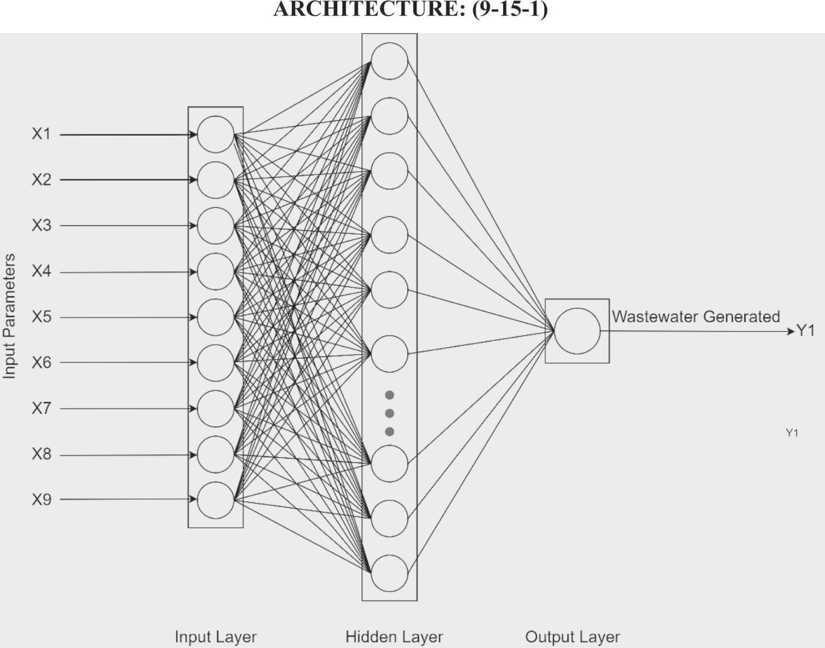
Table 1 shows the input parameters used for the neural network, and Fig. 2 provides a schematic representation of the neural network used in this research.
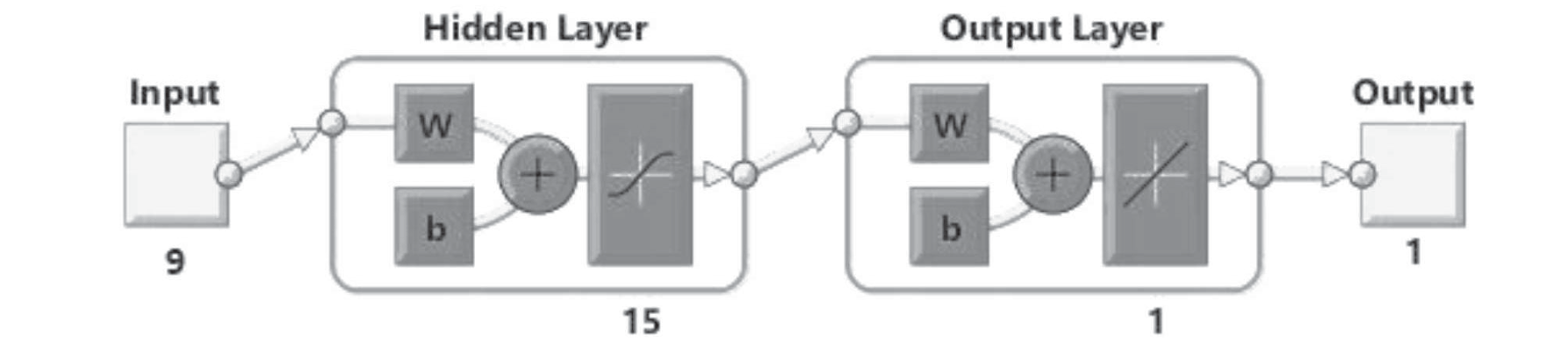
The models developed were made up of three layers: the input, the hidden layer, and lastly, the output layer. The input layer consists of 9 neurons, each representing an input variable. The hidden layer possesses 15 neurons, which were obtained using the best design fit approach. The output layer has 1 neuron representing the output, the wastewater generated. The tansig function represented an activation function at the hidden layer, while the purelin function represented the output layer. The relationship between the input parameters and the wastewater generated is represented by Equation (7).
The mapping between the output and input variables at the hidden layer and output layer can be expressed as follows:
Table 1.
The input variables utilized in this model.
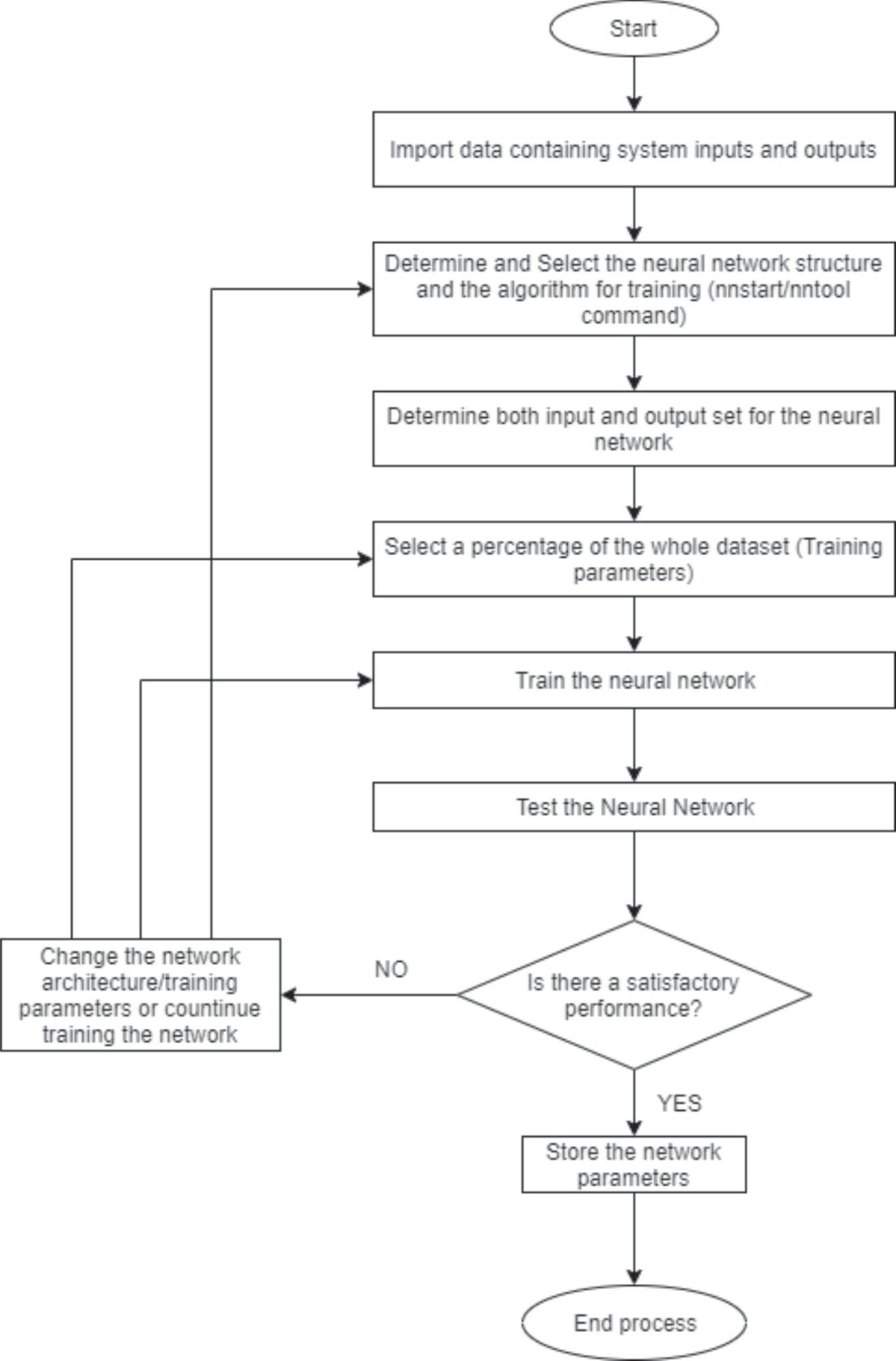
y* represents the generalized output equation of the output layer after several iterations. Fig. 3 illustrates the ANN workflow process from MATLAB. The workflow summarizes the operations that were performed to develop the wastewater prediction model. When the outcomes were less than satisfactory, the network architecture was adjusted.
The network calculates errors on the training and testing datasets. The ANN stops training when the error is minimal, which indicates that the neural network can generalize to an unseen dataset. Performance analysis is based on Regression (R) and Mean Square Error (MSE). Regression analysis is a set of statistical processes for estimating the relationships between a dependent variable (outcome variable) and one or more independent variables (predictors). For any model, the Regression (R) value of 1 is the most desirable, while the R-value of 0 is the least desirable. MSE measures the average of the squares of the errors. It is an error indicator that shows the performance of our model. MSE values closer to 0 are the most desirable.
Results and Discussion
Preliminary Field Investigations
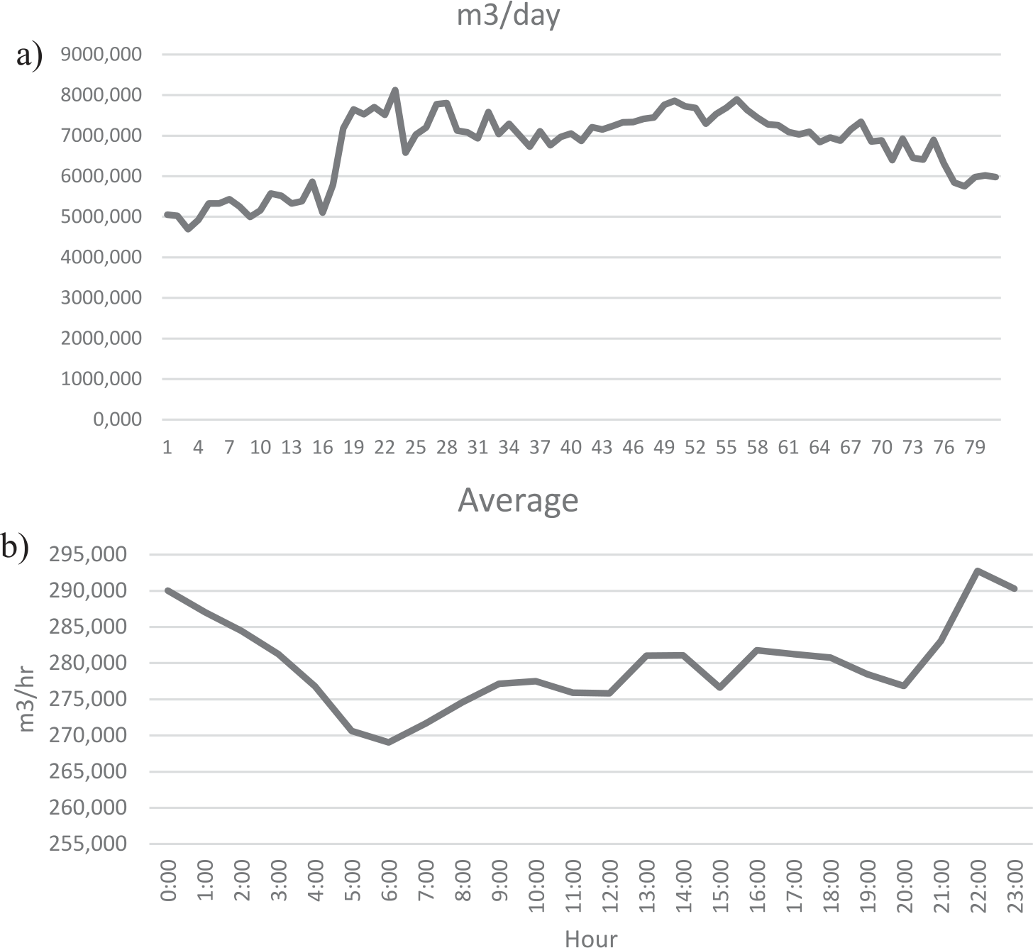
During the 81-day study period, it was observed that an average of 6,724.731 m3/day (6,724,731.019 L/day) of wastewater was discharged into the environment. The peak volume of wastewater discharged into the environment for the study duration was logged at 8125.399 m3 (8,125,399 L). The lowest recorded volume was 4694.240 m3 (4,694,239.897 L). Also, an average of 280.197 m3 (280,000.197 L) of wastewater was discharged from the treatment facility hourly. Furthermore, from field observations, the daily flow rates peaked at about 22:00 h (10:00 pm), with an average flow rate of 293.530 m3/hr. Between 23:00 h (11:00 pm) and 6:00 h (6:00 am), the flow rates declined consistently to a record low of about 269.518 m3/hr. The higher flow at night indicates that water consumption was higher during the night hours compared to the daytime, thus giving an insight into the activities of the university populace. Fig. 4a) and 4b) provide graphical plots of the wastewater volumes recorded during the study period and the graphical representation of hourly flow rates for the duration of the study, respectively.
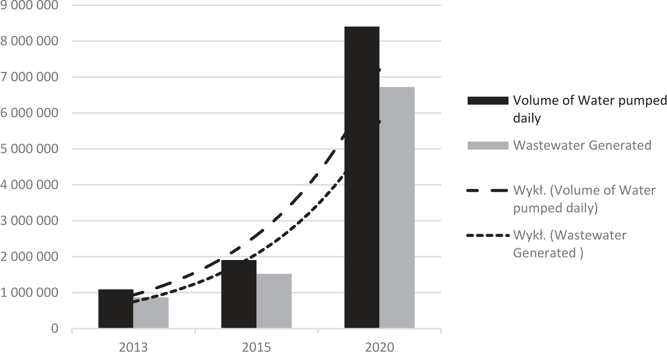
These findings revealed a 339.72% increase in the volume of wastewater obtained from previous studies in 2015 [8, 15]. The wide difference in the values captured in the 2015 and current studies is attributable to using an ultrasonic open channel flowmeter, a precision instrument. The manual method captured wastewater generation data for just a few hours per day over 2 weeks, while the ultrasonic open channel flowmeter was used continuously for nearly 3 months. Fig. 5 gives a graphical comparison of wastewater generated and water pumped within the community for 2013, 2015, and 2020.
Compared to wastewater flows in similar-sized communities, the volumes of wastewater within the campus were similar to USEPA estimates of cities with a similar population. The USEPA estimates that a city of 10,000 people or fewer is expected to generate an average daily wastewater volume of 4,546,092 L a day [16]. The university community has an estimated population of 13,000 residents. However, it receives over 200,000 visitors weekly due to religious gatherings within the city [17].
The volume of water consumed within the community can be estimated from wastewater-generated values because research has shown that 80% of water consumed within a given location is usually transformed into wastewater [1]. Therefore, the volume of water consumed within the campus can be estimated as:
The foregoing implies that for an average of 6,724,731.019 L of wastewater generated within the campus daily, the estimated daily water consumption is 8,405,913.75 L. From these findings, water consumption estimates can be projected for communities globally if population estimates are known. However, variations may exist depending on the unique characteristics of the cities. For instance, residents’ economic, occupational, and social characteristics will significantly affect the water consumption patterns of the community in question.
Prediction Model and Performance Evaluation Using the Levenberg Marquardt and Bayesian Regularization Algorithms
For model development, the 81-day wastewater generation data obtained during field investigations was used to train the model. The structure used for the Levenberg Marquardt and Bayesian Regularization algorithms was (9-15-1). This number was obtained using a heuristic approach. Fig. 6 shows the function-fitting neural network for both algorithms. The developed multilayer perceptron (MLP) model for predicting wastewater generated in the university consists of three layers: the input, hidden, and output layers. Given that the underlying layers have the same structure, the only change here is the training algorithm.
Adapting the same training structure for the Levenberg Marquardt and Bayesian Regularization Algorithms created a similar comparison criterion. The optimum algorithm for the standard wastewater prediction model was determined and adopted.
Testing and Validation of the Developed Model
The parity plots for the volume of wastewater calculated from the neural network against the actual wastewater volumes determined from the 81-day field investigation are given in Fig. 7. The best fit of the outputs (wastewater generated) is represented using colored solid lines, while the dashed lines represent the ideal fit. The hollow circles represent the data. The deviation of the best fit (colored solid lines) and the ideal fit (dashed lines) shows the regression analysis performance evaluation of the model. Fig. 7a) shows the plots obtained using the Levenberg Marquardt algorithm, while Fig. 7b) shows the plots obtained from the Bayesian regularization training algorithm. Fig. 7a) shows the parity plots for the training, testing, and validation stages.
Using the Levenberg Marquardt algorithm, the regression coefficient (R) was 0.911 for the training dataset. This value shows that the Levenberg Marquardt algorithm performs well enough and can predict the volume of wastewater generated. Putting this model to the test, the “external” dataset, initially separated from the rest of the dataset, was used to test the model further to ascertain its performance. The regression plots (R) for both the validation and testing stages are 0.934 and 0.948, respectively, for the Levenberg Marquardt algorithm. The last regression plot for the Levenberg Marquardt algorithm shows that, on aggregate, all the points were located around the bisection; this reveals the accuracy of the result and its capabilities in forecasting the volume of wastewater generated. For the MSE values, the closer the values are to zero, the better. A value of zero means that there was no error in prediction. The Levenberg Marquardt algorithm revealed values of 2.42212×10⁻³, 1.17115×10⁻³, and 3.35980×10⁻³ for the training, testing, and validation stages, respectively. These values show that the algorithm performed well for wastewater volume prediction.
Fig. 7.
Detailed plot of the regression analysis performance evaluation of the model. a) Levenberg Marquardt algorithm, b) Bayesian Regularization algorithm.
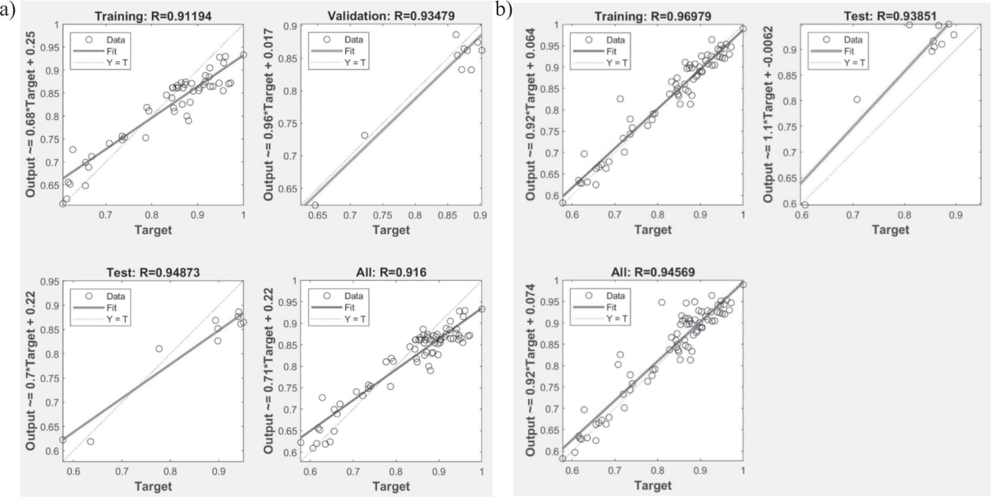
Table 2.
Performance comparison between the Bayesian Regularization and Levenberg Marquardt algorithms.
| Levenberg-Marquardt | Bayesian Regularization | |||
|---|---|---|---|---|
| MSE | R | MSE | R | |
| Training | 2.42212×10⁻³ | 0.91194 | 7.12016×10⁻⁴ | 0.96971 |
| Validation | 1.17115×10⁻³ | 0.93479 | - | - |
| External Test | 3.35980×10⁻³ | 0.94873 | 4.91555×10⁻³ | 0.93851 |
| All | - | 0.916 | - | 0.94569 |
For the Bayesian Regularization algorithm, represented in Fig. 7b), the regression coefficient (R) was 0.969 for the training dataset. This value shows that the Bayesian Regularization algorithm performed well enough and can predict the volume of wastewater generated. Putting this model to the test, the “external” dataset, initially separated from the rest of the dataset, was used to test the model further to ascertain its performance. The regression plots (R) for the testing stage were 0.938 for the Bayesian Regularization algorithm. The last regression plot for the Bayesian regularization algorithm shows that, on aggregate, all the points were located around the bisection; this reveals the accuracy of the result and its capabilities in forecasting the volume of wastewater generated. The aggregate Regression (R) value of the Bayesian Regulation algorithm was 0.945 and was higher than that of the Levenberg Marquardt algorithm at 0.916.
The MSE value for the validation stage in the Bayesian Regularization algorithm was zero, implying no error in the validation stage. Table 2 shows a performance comparison between the Bayesian Regularization and Levenberg Marquardt algorithms.
Extrapolatory Capabilities of Neural Networks
From the results obtained, in terms of regression (R) and mean squared error (MSE) for the models and the external tests, it is evident that the Bayesian Regularization algorithm performed better than the Levenberg Marquardt for wastewater volume prediction. Hence, the Bayesian Regularization model was adopted as the final model. Tables 3 and 4 represent the separated data obtained from the field, which was used to test the Levenberg Marquardt algorithm and Bayesian Regularization algorithms, respectively. The tables present the actual and predicted data, alongside the errors for the separated dataset for both algorithms.
For the evaluation of the extrapolation capability of the developed neural network, the separated data for the remaining 11 days was used as input to the network. The 11-day data was not used for training, testing, and network validation. It was set aside for an external test. An illustration can be taken from day 74 (5th March 2020), which had an actual wastewater volume of 6412.088 m3/day, a predicted wastewater volume of 6651.61 m3/day, and an error of minus (-239.522). On average, the actual wastewater volume was 6268.907 m3/day, the predicted wastewater volume was 6339.455 m3/day, and the error was minus (-70.548) for the separated dataset.
Table 3.
Relationship between the actual and the predicted values of wastewater generated (Levenberg Marquardt algorithm).
Table 4.
Relationship between the actual and the predicted values of wastewater generated (Bayesian Regularization algorithm).
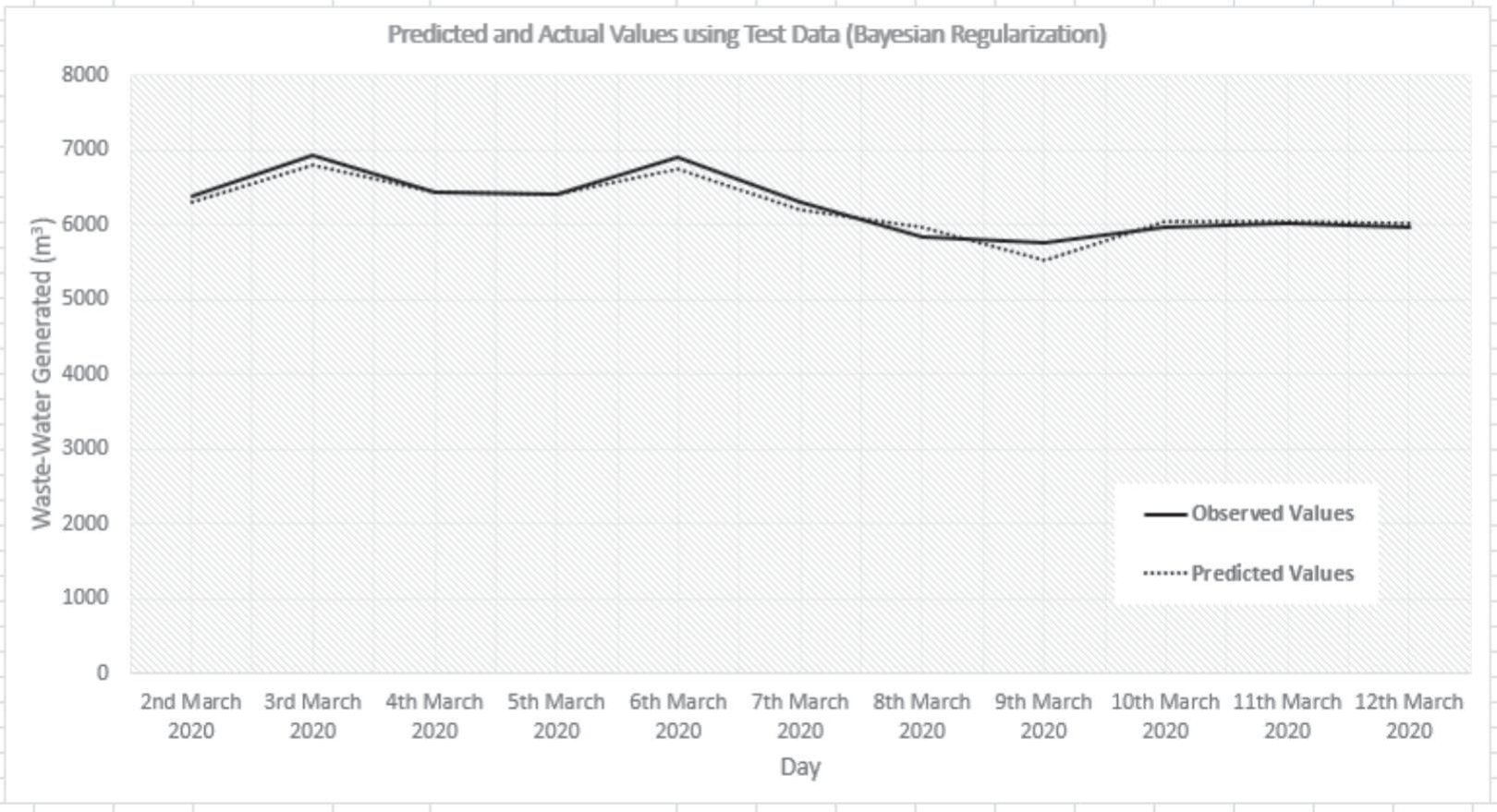
Compared to the Bayesian Regularization, wastewater flows for the same day (day 74) were 6412.088 m3/day for actual wastewater flow and 6420.811 m3/day for the predicted flow, with an error of minus (-8.723). On average, the actual wastewater volume was 6268.907 m3/day, the predicted wastewater volume was 6230.358 m3/day, and the error was 38.549 for the separated dataset. These values further prove that the Bayesian Regularization algorithm performed better than the Levenberg Marquardt algorithm for wastewater volume prediction on the campus.
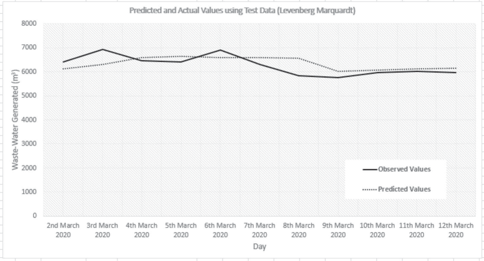
Fig. 8 and Fig. 9 show the graphical relationship between the predicted and observed wastewater volumes for the Levenberg Marquardt and Bayesian Regularization algorithms, respectively. The solid lines on both charts represent the actual values obtained from field investigations for the 11-day separate dataset. In contrast, the dotted lines represent the predicted wastewater volumes for the same period. Given the lack of data for wastewater volumes in similar-sized communities and campuses across the country, the actual-to-predicted data statistics show that the neural network can be extrapolated successfully.
Previous studies have demonstrated the effectiveness of ANN models in making predictions with smaller datasets, which is often the case in most sub-Saharan contexts regarding water and wastewater. For instance, Pasini [18] showed how ANN models could effectively handle small experimental and observational datasets. Literature suggests that the preprocessing of data and structure determination of an ANN model could play a critical role in the efficiency and accuracy of predictions. For example, Yildirim et al. [19] demonstrated that the size of the data set did not impact the accuracy of prediction, which was counterintuitive to the general recommendation in modeling that suggests using the largest dataset possible. Their study found that ANN predicted cotton yield better with 6-year datasets compared to 13-year datasets, which was influenced by the choice of input variables. ANN models can be a reliable option when predicting wastewater volumes for cities that plan to reuse their wastewater or assess the capacities and limits of WWTPs. Additionally, these models help identify opportunities for future research, such as exploring hybrid approaches or alternative architectures to improve performance further.
Systematic Approach to Wastewater Reuse Planning
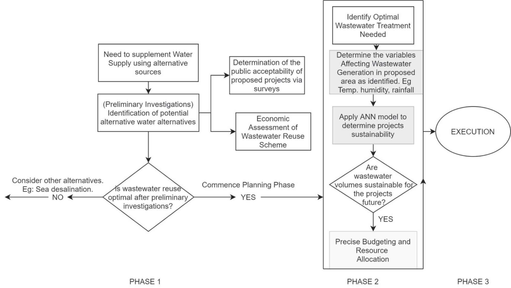
With the low margin of error recorded using the Bayesian Regularization algorithm, a careful adaptation of this model for larger-scale wastewater reuse projects can be critical for higher efficiency. This model can be integrated into planning at university campuses and small and new communities using the input variables as recommended. However, factors affecting wastewater generation may vary depending on the location considered. A wastewater reuse project must follow a systematic approach to attain overall success. This study developed a systematic approach to a successful wastewater reuse scheme. The process is divided into three phases, as identified in Fig. 10. Phase 1 represents the preliminary investigation, Phase 2 represents the planning stage, and Phase 3 involves execution.
Phase 1 (preliminary investigation) will require identification of the needs of the community. These needs will primarily require supplementing any given society’s groundwater or surface water supply. Also, demands for wastewater reuse may occur because of climate change, water, sanitary challenges, etc. Water needs will be identified by carefully analyzing the chosen water supplementary alternatives. At this stage, public acceptability of proposed projects should be carried out alongside economic analysis and evaluation. If wastewater reuse is ideal, it may be safe to proceed to phase 2. In phase 2, the quality of wastewater discharged to the environment should be investigated. However, this phase may depend on the type of wastewater collection system that is operational in the community. Determining the quality of wastewater generated will enable planners to optimize treatment facilities for higher efficiency.
Before applying modeling techniques for wastewater predictions, it is necessary to determine the critical variables that determine wastewater flow. For example, a similar study in Tehran revealed that 11% to 22% of untreated excess wastewater is beyond the capacity of the wastewater reuse system for 2031 to 2040, when climate change was considered [20]. The study found that a 1.29-degree rise in daily temperatures led to a 36.9% increase in daily wastewater generation, implying that certain key variables are critical for developing any wastewater prediction model. A study in northern China reported that less than 24% of rural domestic sewage was treated, hence the need for water consumption and sewage generation data in the area [21]. Their study utilized machine learning models for county-level rural sewage production, which was efficient for sewage treatment designs.
Using machine learning models is advantageous, notably when the model accurately predicts future wastewater levels for the proposed project, allowing for precise budgeting and resource allocation before project execution. Many researchers have tried to utilize machine learning models to predict water quality, but little attention has been paid to predicting the actual volumes of wastewater generated for future scenarios. A combination of quality and quantity in prediction studies concerning wastewater reuse is essential, as one cannot be done without the other. Combining these predictions ensures a holistic approach to wastewater management, improving both efficiency and sustainability. For example, accurate wastewater volume predictions allow treatment facilities to optimize resource allocation (such as energy and chemical usage) while preparing for fluctuations in influent flow, which are often affected by weather conditions or industrial discharges [22]. Simultaneously, wastewater quality predictions enable operators to proactively adjust treatment processes, ensuring compliance with regulatory standards and protecting the environment [23].
For this study, the ANN was integrated into Phase 2 for volume prediction to determine the sustainability of the proposed project. This will enable developers to determine whether future wastewater volumes will sufficiently cater to the project’s needs.
Model Application
The ANN model developed in this study can be adapted for wastewater predictions in small urban cities or campuses with populations between (10,000 and 20,000). The adoption of a population range was to extend the extrapolation of the model to similar-sized campuses. Also, determining the exact number of people residing in communities, especially in developing countries, could be challenging. This study used nine critical variables as input variables for model development. These include the type of day (to provide an insight into the population activities of the residents on campus). Field investigations revealed that the type of day was the most significant factor affecting the volume of wastewater predicted for the community. The second most significant variable that affected wastewater volumes was rainfall. Temperature and humidity had the least effect on flow compared to other variables. However, temperatures caused slight spikes in flows during hot afternoons.
Table 5.
Annotation for the type of day variables.
Given that different campuses may have various factors peculiar to them, the type of day variables were designed to have broad applicability. Several variables may be similar in different universities. For example, Table 5 shows the type of day variables with annotations in ones and zeros. There are situations where a particular day may have one or more defining characteristics, thus determining the volume of wastewater flow.
For this model to be efficient in wastewater prediction in other campuses within the given population range, the type of days peculiar to the given campus has to be identified. For instance, to predict a particular day, one must determine whether the day is a weekday or weekend, a public holiday, a school or business day, and the possibility of a social event or festival within the campus. Identifying these parameters will make for an easy adaptation of the ANN model. Furthermore, the ANN model will be significant for future research within the campus and similar settings. The data will provide information that may be necessary for future studies. Several other predictive tools can be integrated into the system. For example, ANN has been utilized in past studies to determine the performance of a wastewater treatment plant [11, 12].
Conclusions
This study provides a unique insight into how wastewater planners can manage wastewater volumes by predicting the discharge pattern, which, in turn, is determined by empirical characteristics. Information on wastewater generation volumes is significant when considering wastewater reuse schemes. It is also significant in cases where the WWTP receives more wastewater volumes than its design capacity. Due to the increased population and the consequent increase in wastewater volumes, wastewater treatment infrastructure is often overwhelmed. With insufficient funds or land, the possibility of increasing the capacity of the WWTP is nearly impossible. Therefore, the only alternative is the proper scheduling and planning of treatment processes. Although much research has been done on applying ANN to wastewater treatment efficiency, not many studies can be found on the scheduling of treatment volumes, especially in Africa, where there is a paucity of funds for expanding or rebuilding new WWTP infrastructures.
The key findings of this study address three central themes. First, it emphasizes the importance of adequately accounting for generated wastewater volumes and the intricate and unique parameters contributing to their variations in different contexts and locations. To ensure proper accountability, accurate measurements and regular data collection and archiving must be done. Secondly, the study demonstrated the impact of user characteristics on wastewater generation patterns. This may vary from location to location. Adequately capturing these variations will have a significant impact on the accuracy of the prediction model. Thirdly, the study promoted the merits of wastewater reuse in contrast to the continuous withdrawal of freshwater from groundwater sources. Further, the study proposed a three-phase systematic approach for planning a wastewater reuse project.
While this study focused on a small university campus wastewater management scheme, it has significant implications for large-scale applications. In environments where freshwater constraints exist, the available generated wastewater has the potential to become a valuable resource. However, further research needs to be done to improve wastewater volume prediction and treatment efficiency. This research contributes to the modelling framework for achieving the fundamental objective of proper volume measurement and prediction.
The limitations of this study constitute the basis for future research. For example, year-round data collection and a detailed hourly analysis of collected data can give a more robust and accurate prediction model. Further research into wastewater volume accountability is necessary to protect the environment and promote the practice of freshwater conservation and sustainable extraction.