

Introduction
Contemporary human activities, including industrialization, urbanization and the constant expansion of economic scale, negatively affect both natural resources and the environment as China enters its rapid development stage [1]. From the 1990s- 2012, China’s sustained high economic growth relied on the disorderly, rapid and massive consumption of nonrenewable resources and energy, which has led to many ecological and social security problems [2]. Development in areas where resource depletion and environmental pollution coexisted was severely hampered. Until the growing significance of the eco-environment for sustainable economic development was recognized, local and national governments attached importance to ecological issues and strengthened related management. After decades of development, new philosophies and goals, including ecological civilization [3], the beautiful China initiative and green development, were incorporated into the “Constitution of the People’s Republic of China,” which provides solid political foundations for eco-environmental protection [4]. The implementation of other national strategies and policies also offers strong support. For instance, China’s provincial carbon peak and carbon neutrality actions have clarified the available path for ecological conservation and environmental load alleviation [5, 6].
Hubei Province is one of the most dynamic heavy industrial regions in China and a key experimental area that is positively engaged in economic transformation. During the 20 years before and after the beginning of the 21st century, the heavy chemical enterprises located in Hubei Province resorted to a crude development approach against the background of vigorously promoting urbanization and pursuing high growth as measured by economic indicators. Consequently, some cities in Hubei Province, particularly Huangshi, Ezhou and Daye, suffered from serious ecological damage and a resource depletion crisis. Furthermore, environmental pollution has caused substantial economic losses. Increasingly aggravated contradictions among regional development, ecological environment and natural resources urgently need to be addressed in these areas by improving eco-efficiency or reducing environmental loads [7, 8]. Starting in approximately the 2010s, the provincial government took measures to decrease high environmental loads to achieve sustainable economic growth and improve resident living standards, with the goal of promoting ecological restoration and green development. Moreover, heavily polluting enterprises were urged to increase their levels of capital investment in environmental protection and treatment and promote technological upgrades and equipment transformation to reduce pollution emissions and environmental contamination risks. Especially under the context of China’s commitment to advancing the harmonious balance between the construction of eco-environmental protection and economic development during “the 14th Five-Year Plan” period (2021-2025), Hubei Province desperately needs to alleviate the pressure of environmental loads. Thus, it is necessary to evaluate the environmental load level of Hubei Province in recent decades and present corresponding policy recommendations for its future sustainable and high-quality socioeconomic development.
Environmental loads were developed in commercial fields and then defined by scholars in accordance with different research objects. Several representative definitions are presented below. The concept of environmental loads was originally used to describe the pressure created by the quantity and variety of individual entrepreneur information that are simultaneously processed when working in an environment comprising uncertainty, complexity, deadlines and the anticipated consequences of actions [9]. Nijdam et al. (2005) introduced the concept of environmental loads into a private consumption study and defined the direct environmental load as the load that occurs during product use by consumers [10]. This was distinguished from the indirect environmental load, which is the load that occurs before the product or service has been purchased and after it has been collected for waste treatment. Det Norske Veritas (2010) pointed out that environmental loads are loads caused by environmental phenomena and are generally determined by the structure, size, shape and response characteristics of enterprises and institutions [11]. Then, Wang (2017) and Zhang (2021) each suggested that environmental load reflects not only the combined impact of the study objects, such as human production activities, lifestyles and consumption behaviors, on natural resources or the eco-environment but also the change intension of a natural ecosystem after receiving pollutant emissions compared to its initial state [12, 13]. Liu et al. (2022) and Zhang et al. (2023) used environmental load to refer to the combined value of the resources and energy consumed and the waste discharged into the environment during the material production process [14, 15]. The established concept of environmental loads focuses on environmental impact. In this study, we describe ecological loading as the combined impact of stress and burden on the environment that originates from pollution discharge arising from the resource and energy consumption of various human activities.
Achievements in assessing the environmental loads have been conducted to this day. Environmental load assessment is a comprehensive procedure that generally involves multiple types of influencing factors and involves quantitative evaluation and analysis [16, 17]. Depending on the research objects and contents, the impact factors in environmental load evaluation can be classified into several categories. For example, Lin (1999) and Fang (2016) selected air pollutants (including NOx, SOx, soot and dust, etc.), water pollutants (including sewage, chemical oxygen demand, etc.) and solid wastes as the valid indicators involved in energy consumption to analyze the environmental loads of paperboards and buildings during their life cycle [18, 19]. Sasongko et al. (2018) assessed the environmental load of continuous bioenergy production using material and energy balances, greenhouse gas (GHG) emissions, nutrient requirements and water scarcity during the bioenergy production cycle [20]. Significantly, many researchers [21-25] selected influencing factors based on resource consumption (e.g., steel, aluminum, cement, construction glass, wood, concrete, etc.), environmental pollution (e.g., CO2, CO, CH4, N2O3, etc.) and energy consumption (e.g., fossil fuels, electricity, etc.) to establish environmental load evaluation systems and study the quantitative relationship between economic growth and environmental loads. Salman and Hasar (2023) newly classified environmental problems under four main headings: water, waste, air and traffic [26]. Notably, most of these studies classified environmental loads into three categories: resource environmental load, energy environmental load and waste environmental load. Accordingly, environmental loads that affect those factors directly caused by human activities have been classified into energy and resource consumption, environmental pollution, ecological destruction, waste discharge, etc. Among them, the discharge of waste gas, wastewater and solid waste are always considered the most significant and key indicators, as they induce regional environmental pollution and environmental load increases. Therefore, factors, including sewage, waste gas and waste aspects, can be summarized as major influencing concerns in environmental load assessment.
Simultaneously, it is worth pointing out that related analytical approaches provided important supplements and have been constantly optimized. For example, Agostinho and Pereira (2013) [27] and Liu et al. (2015) [28] separately adopted the emergy ecological footprint and equivalent factors to measure regional environmental loads. Gao and Zang (2017) applied an exponential model to comparatively analyse and comprehensively evaluate scheme of environmental loads [29]. Tian and Shen (2019) utilized niche suitability to evaluate the provincial eco-environmental loads and associated response to industrialization [30]. Cui and Zhang (2019) used regression analysis to explore the relation between the regional environmental load and regional economic growth [31]. Zhang et al. (2023) carried out spatial autocorrelation analyses, kernel density estimation analyses and the logarithmic mean division index (LMDI) methods to identify the areal distribution and temporal variation in carbon emissions of public urban buildings [32]. Among them, the gray correlation analysis which is proposed by Professor Julong Deng in 1982 offers an important process to this study.
The gray correlation analysis, as the basic content of gray theory, is a multifactor statistical method based on the relationships [33, 34]. Specifically, it is used to measure the convergence of the dynamic change trend among factors in the analyzed system, namely, the gray correlation grade [35, 36], to reflect the full status of affairs [37] in a time series. This quantitative comparative analysis objectively shows the matching performance between the actual and expected values. Because the gray theory has strength in addressing systematic problems such as small sample sizes, poor information and uncertainty [33], it can be used in modeling when atypical data distribution patterns and limited information for sample analysis are present. Meanwhile, the calculation results are highly explanatory, stable and consistent with the actual state [38]. Besides, the gray correlation analysis method takes the synthesizing evaluation of situations or phenomena that are affected by multiple factors from a holistic perspective [38] and compensates for the defect of the regression analysis method, which reduces the accuracy of analysis when data are lacking. Bias related to the subjective tendencies of experts are mostly avoided to ensure objectivity of results. Developed during the past 40 years, this method or the derived methods have been widely applied in fields such as land resource evaluation [39, 40], regional development evaluation [41, 42], urban transportation [43, 44], as well as environmental impact assessment to ensure good results and benefits. Continuous progress in modeling and analyzing environmental loads has been made using the gray evaluation theory. For example, Shi and Xia (1997) introduced the gray-mode identification model to evaluate water quality via the relational discrepancy degree and the gray subordination degree [45]. Xu et al. (2011) presented the waste-discharge pollution state and evaluated the environmental pressure that was generated from power plants [46]. Lu et al. (2013) [47] and Zhao and Feng (2022) [48] characterized the evolution trend of energy consumption’s impact on the environment and provided scientific strategies for China’s environmental decompression and energy structure adjustment via gray correlation degree. Ren et al. (2017) [49] and Wu et al. (2018) [50] used the gray correlation analysis model to determine the influence of industrial energy consumption on the atmospheric environment or the leading causes of decoupling indices differences from different perspectives. Huang et al. (2019) [51] calculated gray relational grades to identify the indicators of energy consumption that are strongly correlated with carbon emissions. Zhang et al. (2020) [52] and Niu et al. (2022) [53] quantified difference degrees and extracted the main elements affecting the ecological interior conditions or the cities’ sustainable development capability by using the gray correlation analysis. Tao et al. (2022) [54] analyzed the pollution of river environments by combining gray relational analysis with an analytic hierarchy process and entropy weight method. Clearly, existing studies concentrate on the environmental burdens generated by energy consumption. And few concern the variation tendency through comparing the internal factors of the system or the close connection between environmental pollution and economic development policy. In order to know the development profile of system elements, the mathematical abstract method of correlation analysis is valid using reference-actual values. Briefly, the feature of the gray correlation degree assessment model is consistent with the research objective of eco-environmental loads. The gray correlation analysis process is applicable for evaluating environmental loads.
The objective of this article is to measure the environmental loads with typical influencing elements using the gray correlation degree analysis to assess the variation tendency and analyze the system’s health in Hubei Province during 1995-2019. Corresponding countermeasures are proposed for concurrently improving ecological suitability and maintaining ecosystem balance.
Material and Methods
Study Area
Hubei Province is in central China, with a total area of 185900 square kilometres, of which mountains, hills and plains and lake areas account for 56, 24 and 20%, respectively. Located in the transitional climatic zone from north to south China, Hubei Province has a subtropical monsoon climate characterized by cold winters and hot summers. The annual average temperature is 15-17ºC. The annual average precipitation is 800-1600 mm, with distinct seasonal variations in precipitation distribution. The total population maintains low and steady growth, attaining a resident population of 58.3 million by 2021.
Moreover, the equipment manufacturing industry, which is one of the old industrial bases in China, is an important pillar industry of Hubei Province. With the rapid development of the economy, Hubei Province has come under pressure from resource scarcity and serious eco-environmental pollution driven by a high proportion of primary industry, a low level of agricultural modernization and an increasing discharge of pollutants. To address the noticeable problems of air pollution, water pollution, garbage waste contamination and soil pollution, Hubei Province has actively implemented measures and carried out special rectification activities meant to comprehensively and continuously improve the level of environmental quality.
Choice of Impact Indicators and Data Sources
Based on previous research and relevant standards, industrial pollutant emissions are emphasized in this paper, and indicators are selected for environmental load evaluation from three aspects: waste residue, exhaust gas and wastewater. In the context of the carbon peaking and carbon neutrality goals, the carbon emission impact factor is introduced as needed. Specifically, these seven selected factors are the total wastewater discharge, industrial solid waste emission, industrial wastewater emission, industrial waste gas emission, sulfur dioxide discharge, industrial soot and dust discharge and carbon dioxide emission.
The data sources are the Annual Statistical Bulletin of National Economic and Social Development in Hubei Province [55] and Hubei Provincial Statistical Yearbook during 2001-2021 [56]. Among them, the CO2 emission data cannot be obtained directly from statistical yearbooks since its statistical work at the provincial level is late. It is calculated according to the total energy consumption and the carbon emission coefficient of standard coal, which is 2.89 kgCO2/kgce per the reports proposed by the Intergovernmental Panel on Climate Change (IPCC) and the actual situation in Hubei Province [57, 58].
Steps of the Gray Relational Analysis Method
The main procedures for establishing the gray correlation degree model involve constructing an index system; determining the analysis series; applying dimensionless processing; and calculating the absolute differences, correlation coefficients and correlation degrees. Finally, the environmental load level is determined and analyzed. The following subsections present the detailed steps of this process.
Constructing the Analysis Index System
According to the gray system theory, all factors influencing the environmental loads detailed above are regarded as a gray system. Suppose there are m evaluated years used as alternatives and n evaluation indexes used as attributes for the gray system. The analyzed data can then form the following matrix:
(1)
where G is a data set of the determined evaluation system composed of m alternatives and n indexes; m denotes the total number of years to be evaluated, where m = 22 in this study; n denotes the number of parameters for environmental loading evaluation, where n = 7 here; gij denotes the observation value of factor j at the evaluated year i; and Gi is the ith alternative and represents the ith data series of a subsystem, which is defined as Gi = (gi(1), gi(2),…, gi(n)).
The determined analysis system constructs the space of the gray message relation for our objective in this paper.
Determining Analysis Sequences
The gray correlation analysis adopted for this study is better at quantitatively analyzing the development trend of a dynamic process through the estimation of the geometric relations in the system. Determining the analysis sequences, including the comparison sequences and reference sequence, is essential for measuring the relationships between subsystems based on the collected statistical data.
A comparison sequence, as one sample object, is a data sequence composed of performance indicators that affect the system’s behavior [34]. The index sequences denoted as G1, G2,…, Gm are specific evaluation targets in the factor set G, which is composed of time scales.
The reference sequence is a data sequence that reflects the characteristics of a system’s behavior [34]. According to the feature of variables selected, the maximum value of each indicator in the matrix of evaluation indexes is selected to form the reference series. This paper defines the reference state as follows:
where G0 denotes the reference sequence and gi(k) stands for the largest value of the jth variable among gi(j).
Dimensionless Transformation of Variables
Normalizing the raw data is a necessary step in gray relational analysis. The original data are expressed in different measurement units and must be standardized to make these measurements comparable and enhance the reliability of the evaluation results. Depending on the characteristics of the original sequences, the environmental loading indicators used in this paper have a relatively single attribute, namely, the equalization method employed for data preprocessing. The reference series and comparison series can be normalized as follows:
where gij' stands for the transformed data; thus, the transformed set can be expressed as G' = (gij')m×n; gj is the average value of the jth variable with raw data; g0'(k) is the preprocessed reference value, g0'(j) = g0(j)/gj, j = 1, 2,..., n; and Gi' and G0' denote comparison sequences and the reference sequence after preprocessing, respectively.
Calculating the Difference Series, Minimum and Maximum Differences
Next, the absolute difference between the reference value and the comparable value can be calculated one by one using Eq. (7). Consequently, the difference series can be obtained with Eq. (8). These deviation series form the differential matrix. The minimum and maximum differences are determined in Eq. (9) and Eq. (10).
where Δi(j) is the absolute difference value between the dimensionless reference value and the comparability value; Δi is the ith deviation sequence; and a and b are the smallest and the largest values in the deviation matrix, respectively.
Calculating the Gray Correlation Coefficients
The gray relational coefficient is used to reflect how close the reference series and the comparability sequence are. The calculation formula is:
where ξi(k) is the correlation coefficient with the range of (0,1]; ε represents the resolution coefficient within [0,1] and is often taken as 0.5 [59].
Calculating the Correlation Degree
As we have considered that each of those seven indexes exert the same effect on the system of ecological load evaluation in Hubei Province, the correlation grade obtained between the reference series and the comparability series can be derived from the following formula.
where ri is the gray relational degree. The greater the correlation degree is, the higher the similarity is between the comparison year and the reference sequence in the analysis system, and vice versa. According to the magnitude of the correlation, the evolution trend of environmental loads in Hubei Province can be evaluated by years.
Results and Discussion
Collection of Raw Data
The evaluation indicators detailed above were used to measure the level of environmental pollution loading in Hubei Province from 1995 to 2019. The initial collected data are shown in Table 1. These raw data form an index system according to Eq. (1). The maximum data in the initial sequence Gi constituted the reference series using Eq. (2).
Data Processing
First, the original observation number of the evaluation index is made dimensionless. Based on the data in Table 1, the standardized value of each variable is calculated through Eqs. (3)-(6). The results are shown in Table 2.
Then, the difference matrix is found using Eqs (7)- (8). Additionally, we obtain Table 3.
Next, we find the two poles among the difference values with Eqs (9)-(10). Then, we have Table 4.
Finally, the correlations of environmental load factors are obtained through Eq. (11); the arithmetic mean of correlation coefficients can be obtained as the gray correlation grades that are associated with each factor using Eq. (12), as shown in Table 5.
Table 1.
The original sequences for conducting environmental loading evaluation in Hubei Province.
Table 2.
Comparison and reference sequences after data preprocessing.
Table 3.
Absolute difference value (∆i(j)) of Gi compared with G0.
Table 4.
Minimum and maximum differences of indexes.
According to the size of the correlation grades displayed above, the variation trend of the environmental loading state in Hubei Province from 1995-2019 can be drawn in Fig. 1. Concomitantly, we obtain Fig. 2 by calculating the arithmetic mean of each factor.
Results
As shown in Fig. 1, the gray correlation degrees of eco-environmental loads in Hubei Province during 1995-2019 were generally high, with an average value of 0.726. The environmental loads peaked in 1999 and 2011. The overall level of environmental loads in Hubei Province showed a slow and fluctuating decrease from 1995-2019. Simultaneously, there were significant differences detected in the integrated correlations of environmental load factors, which are analyzed as follows.
Fig. 1.
Gray relational grades for the comparability sequences of the environmental loads in Hubei Province during 1995-2019.
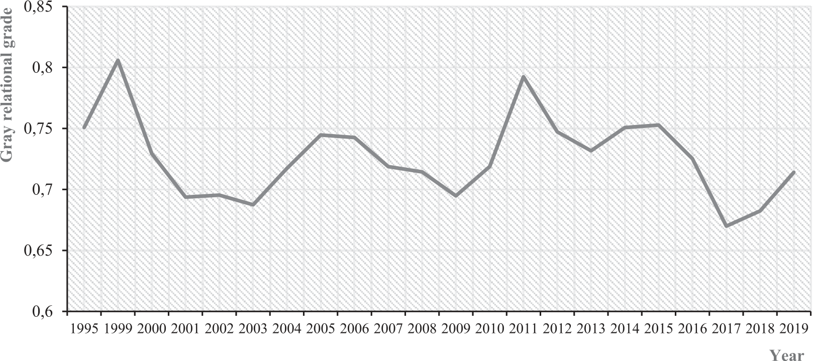
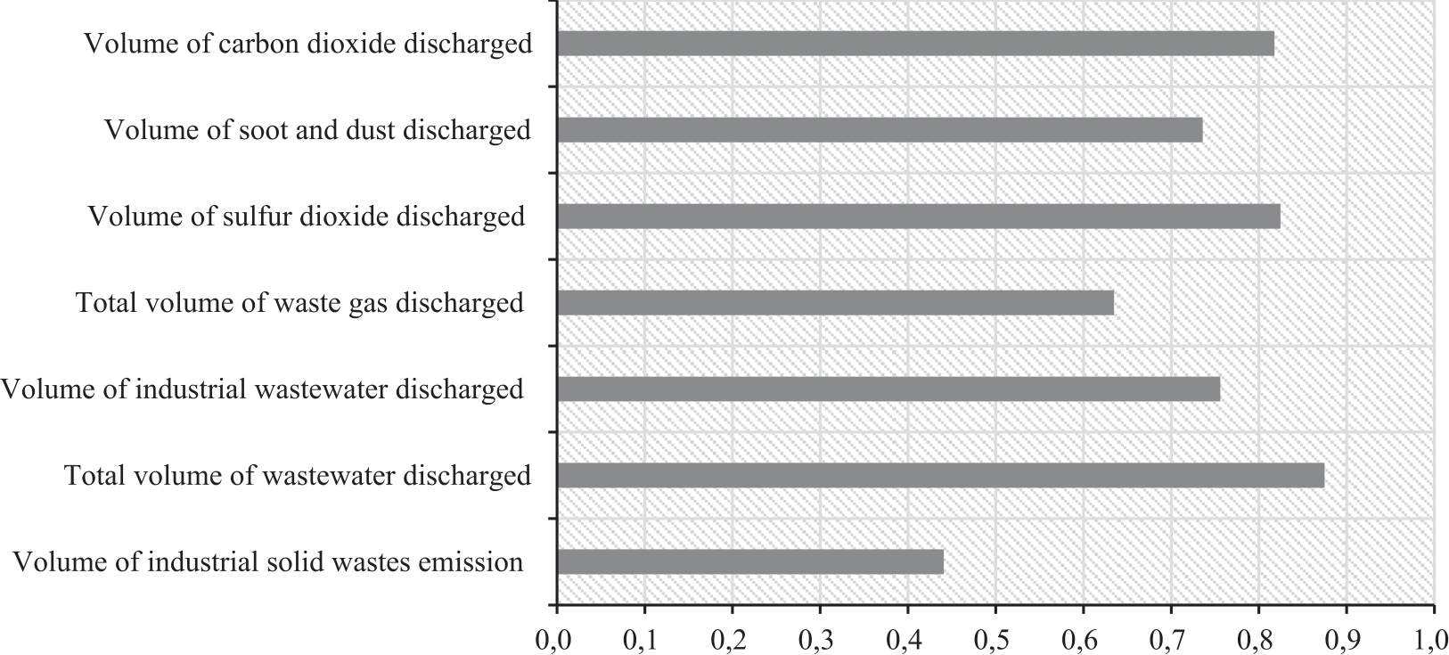
Table 5.
Correlation coefficients of evaluated years with the reference column.
From 1995 to 2003, the level of environmental load in Hubei Province first increased and then decreased, indicating that it was high at the beginning of this period and then decreased significantly following a period of improvement. The concrete analysis is described in further detail below. 1) In the 1990s, the environmental load in Hubei Province showed an upward trend with a severe state that peaked in 1999. The appearance of this characteristic can be attributed to the following three aspects: (a) before 2000, as an old base for the heavy chemical industries, Hubei Province had an abnormal industrial structure with secondary industries that were characterized by excessive pollution and energy consumption; (b) in the late 1990s, weak national awareness of environmental protection and a lack of relevant policies at the legal or industrial regulation levels could not effectively restrain environmental damage behaviours; and (c) poorly developed technologies limited the efforts to reduce pollutant discharges. 2) Accompanied by a slowdown in the growth of total pollutant emissions, the environmental load in Hubei Province gradually decreased from 1999 to 2003. This can be mainly attributed to the following reasons: (a) governmental agencies, enterprises and public institutions increased the importance given to environmental protection and actively carried out studies on sustainable development and the circular economy. This was accompanied by a gradual improvement in national environmental legislation after the beginning of the 21st century. (b) Hubei Province implemented a series of management policies and systems, such as levying compensation taxes on resource development for ecological construction since 2001. This was done in response to the explicit directions on eco-environmental protection as a fundamental entry point for the large-scale development of western China.
From 2003 to 2011, the eco-environmental load in Hubei Province fluctuated and rose, indicating that the overall eco-environmental system was unstable. This was accompanied by discordance between the regional eco-environment and economic development. Specific analysis is provided below: 1) From 2003 to 2005, Hubei Province experienced a slight rebound and increase in its environmental loads. This was due to the release of pollution impacts on the environment under the driving of economic goals. 2) From 2005 to 2011, the environmental loads first decreased steadily and then increased rapidly. Therefore, (a) the environmental load in Hubei Province declined continuously, as did the level of eco-environmental load correlation from 2005- 2009. The reasons for this are as follows. First, Hubei has been eliminating and rectifying those industries with inefficient production capacity and high pollution since the strategic initiative of revitalizing national old industrial bases was proposed in 2003. Second, China widely popularized innovative technology usage for environmental governance, such as secondary treatment technology for industrial wastewater and industrial desulfurization and denitrification technologies, which has greatly reduced the emission of industrial pollutants and helped avoid the path of pollution first and governance later. Third, after the Copenhagen climate summit in 2009, the principle of a low-carbon economy was adopted by the government as a means of energy savings and carbon reduction. Furthermore, most cities in the province were actively engaged in low-carbon construction, especially in response to the goal of reducing carbon dioxide emissions per unit of GDP by 40-45% by 2020 compared with 2005. (b) From 2009- 2011, the environmental load in Hubei Province rose rapidly, experiencing a brief upturn in its correlation grades. This increase was due to the fast pace of the overall growth of the regional economy from 2005-2009 and the increasing GDP growth rate year by year. The second was because the progress of industrial structure optimization and upgrading had slowed. The proportion of the secondary industry remained high, especially that of the heavy chemical industries, which accounted for a large amount of the output value and pollutant discharges.
From 2011 to 2019, the overall level of eco-environmental load in Hubei Province showed a downward trend with fluctuating changes. The fluctuating decline was due to, on the one hand, the national emphasis on green and ecological civilization construction under the goals of carbon peaking and carbon neutrality with no reliance on resource and energy consumption for rapid economic development. On the other hand, in 2015, China committed to the world that it would reduce its carbon dioxide emissions per unit of GDP by 60-65% by 2030 compared to that in 2005. Notably, the slight increase from 2017 to 2019 was mainly due to the large total amount and intensity of emissions, which made pollution prevention and control extremely difficult in the current historical stage with rapid economic and social development. Moreover, because the promotion of emission reduction technologies caused aftereffect inadequacy, many enterprises relaxed their vigilance against adverse impacts caused by the increase in the quantity and variety of pollutant emissions on the environment. This was done in pursuit of output value and profits after having experienced a short period of constraint from a low-carbon economy. In turn, this was influenced by the following context: first, the proportion of energy-intensive industries in the added value of industries above a designated size in Hubei Province rose from 26.8% in 2015 to 29.2% in 2020. Second, the ratio of coal-based fossil energy consumption to total energy consumption remained above 80% for a long time, with an underdevelopment of resources such as hydropower, wind power and photovoltaics. Third, the proportion of highway freight volume exceeded 70%. Finally, the policy framework and institutional mechanism for achieving a carbon peak had not yet been formed.
In sum, the results obtained by the gray correlation degree analysis method are consistent with the observed trend of environmental load changes in Hubei Province. The high correlation grades of environmental loads indicate a relatively strong relationship with socioeconomic development. Additionally, wastewater, SO2 and CO2 are the main environmental load influencing factors in Hubei Province according to the correlation sequence of each factor (see Fig. 2).
Discussion
The environmental load in Hubei Province has undergone stages of peak load, fluctuating decline and rebound over the last 20 years. This has been closely related to the industrial structure, economic development, innovation technology and social participation in the current period. Following measures were proposed to alleviate the eco-environmental load and enhance the overall health conditions of the ecosystem in Hubei Province.
First, environmental infrastructure optimization helps reduce the gap between eco-environmental governance and modernization requirements to prevent ecological risk. The construction of monitoring networks makes eco-environmental governance more scientific, refined and informationalized. In particular, it is necessary to control the spatial transmission effect of industrial pollution, establish regional joint prevention and control mechanisms for the atmospheric environment and formulate environmental governance standards for regional industries. Additionally, the optimization of economic and legal means and market-oriented mechanisms such as product value realization and green finance contributes to the guidance of industrial enterprise development in harmony with the eco-environment in Hubei Province.
Second, adjusting the industrial structure and increasing the proportion of technology-intensive industries help enhance the green and low-carbon transformation of Hubei Province. Close-out and transformation are basic paths for the overall upgrading of enterprises with high pollution and energy consumption in the steel industry, manufacturing, mining and heavy chemical industry. Meanwhile, the auditing mechanism for cleaner production facilitates clean and energy efficiency improvements. Moreover, policy guidance for energy level upgrading should be strengthened to promote the integration, clustering and ecologicalization of strategic emerging industries, such as digital creative industries.
Third, green technology innovation supports the decrease in environmental loads in Hubei Province. Heavy industries should actively carry out technological innovation in energy conservation and emission reduction. The formulation of strategic plans from the aspects of talent cultivation, patent protection, incubation and application of achievements enhances the penetration of innovative technologies in eco-environmental governance. The key players in technological innovation can be expanded under the support of national demonstrative bases. The East Lake National Innovation Demonstration Zone has been taken as the core to exploit the scientific research advantages of universities and promote industry-university-research institution cooperation in Hubei Province. So it is necessary to develop new modes of services for enterprises and promote the exchange and cooperation of innovative technologies.
Fourth, universal participation deserves recommendations. The widespread recognition of environmental protection and ecosystem balance in community colleges as well as exhibition and publicity activities raise the public’s participation enthusiasm and responsibility consciousness. Due to the severe situation of resource constraints and environmental pollution, the construction of ecological civilization should be integrated into the whole process of socioeconomic development. The creation of a common governance system with government as the leader, enterprises as the main body and public participation offers an immensely synergy for universal participation in high-level eco-environmental protection and construction while reducing the environmental load in Hubei Province.
Conclusions
In this paper, the gray correlation degree method is adopted to evaluate the change trend of the environmental loads in Hubei Province, China, and to provide effective suggestions for eco-friendly and sustainable development. The environmental loads over the past two decades have shown a fluctuating decreasing trend, but the load level was generally high and accompanied by prominent problems of sewage discharge and exhaust gas emission. Consequently, the ecological and environmental quality in the Hubei area urgently needs to be continuously optimized. The government should focus on solving and controlling the pollution problems caused by sewerage, exhaust gas and waste residue during the implementation of the 14th Five-Year Plan. Furthermore, reforming eco-environmental protection and management mechanisms by establishing a system of paid use for natural resources is a positive means for alleviating environmental loads.
The method used in the study is relatively simple and easy to extend and apply in other fields related to environmental quality evaluation. The use of data samples with a long time span reduces the contingency and makes the comprehensive performance assessment feasible. However, from the results, we can see that the gray correlation degree analysis method tends to be homogenized with low resolution. Hence, the applied method needs to be further improved by overcoming this shortcoming for more precise evaluation information. In addition, rather than selecting some representative indicators for regional eco-environmental load evaluation, future research can further enrich and verify them from other aspects.