

Introduction
With accelerated urbanization and rapid economic development, fossil fuel consumption such as coal and oil increased substantially, causing serious fine particulate matter (PM2.5) and ozone (O3) pollution in China [1-3]. Atmospheric O3 is mainly distributed in the upper stratosphere and troposphere. Stratospheric O3 protects human health and the Earth’s ecosystem by resisting ultraviolet light and insulation [4-6]. Surface O3 is partially derived from stratospheric O3 seepage and mostly from anthropogenic pollution such as emissions from motor vehicles and petrochemical industries [7- 9]. O3 is a secondary air pollutant, mainly produced by nitrogen oxides (NOx) and volatile organic compounds (VOCs) through a series of photochemical reactions [10, 11]. Due to the irritating and strong oxidizing properties of O3, high O3 concentrations damage human health and the ecosystem [12]. Serious O3 pollution has drawn much attention from the scientific community and the government [13-15]. Some studies revealed that hundreds of thousands of people die each year from respiratory diseases caused by O3 pollution in China [16, 17]. Additionally, O3 pollution is involved in crop photosynthesis and inhibits crop growth [18-20].
Numerous studies have shown that the type of air pollution in China is shifting from PM2.5 to O3. The synergistic effects of O3 and PM2.5 make air pollution more difficult to control [21-23]. Recent studies about O3 pollution have focused on spatial and temporal variations, influencing factors, and effective control measures [24- 26]. In the past few years, the O3 concentration has been on a slow upward trend in China [27]. In some cities, O3 has become the primary pollutant during the warm seasons [28, 29]. In recent years, O3 pollution-related studies in China have mainly focused on economically developed regions such as Beijing-Tianjin-Hebei (BTH-UA), the Yangtze River Delta (YRD-UA), the Triangle of Central China (TC-UA), Chengdu-Chongqing (CY-UA), and the Pearl River Delta urban agglomeration [30]. Few studies have been aimed at the O3 pollution in the HREB. The HREB is in eastern China, with a population accounting for 10% of the national total population. In addition to being an important grain-producing area in China, the HREB also has many industrial cities, including Rizhao, Zhengzhou, Fuyang, Bengbu, Linyi, Yancheng, and Xvzhou [31, 32]. Liu et al. found that both meteorological conditions and precursor emissions affect ozone concentration changes in the Huaihe River Basin [33].
This study aimed to investigate the spatial-temporal distribution and meteorological driving forces on O3 variation in the HREB by using a multi-method approach, specifically: (1) the annual, seasonal, monthly, and diurnal variations of O3 concentrations were systematically described’ (2) the spatial variation of O3 was analyzed; and (3) the meteorological driving forces were estimated. The study results contributed to a further understanding of the spatial-temporal patterns and mechanisms of O3 pollution in the HREB. Further, the findings provided a scientific basis for the O3 control measures in the HREB.
Materials and Methods
Study Area
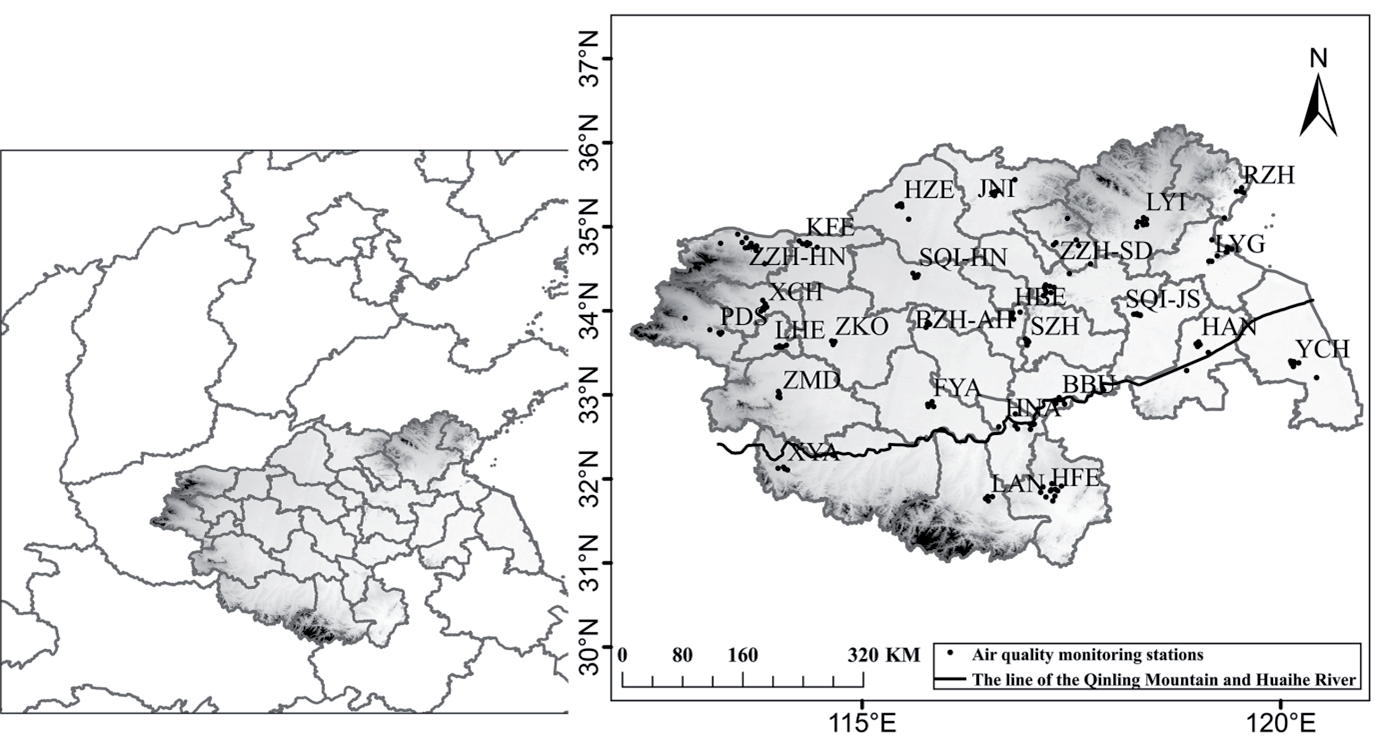
The HREB (30.9°N-36.2°N, 112.2°E-121.0°E) is located in central China (Fig. 1), including 27 cities: Luohe, Pingdingshan, Xuchang, Xinyang, Zhoukou, Zhumadian, and Zhengzhou in Henan Province, Bengbu, Bozhou, Fuyang, Huaibei, Hefei, Huainan, Luan, and Suzhou in Anhui Province, Heze, Jining, Linyi, Rizhao, and Zhaozhuang in Shandong Province, Huaian, Lianyungang, Suqian, Xvzhou, and Yancheng in Jiangsu Province. Among them, Zhengzhou is the capital city of Henan Province, with a huge population [34]. As a resource-based industrial city in Henan Province, Pingdingshan has abundant coal resources. Hefei, the capital of Anhui Province, is one of the megacities in China. Xuzhou is an important coal and power production area in China. The HREB covers about 205, 000 km2 with a population of about 180 million [35]. The line of the Qinling Mountain and Huaihe River is the boundary between the temperate and subtropical zones of China, as well as between the subtropical and temperate monsoon climates.
Materials
Hourly O3 mass concentration data from 2015 to 2020 was obtained from the China National Environmental Monitoring Centre, published by the Ministry of Ecology and Environment of the People’s Republic of China. The daily maximum 8-h sliding average of O3 concentration (MDA8-O3) was used to represent the daily average O3 concentration. Meteorological data, including temperature, pressure, precipitation, wind speed, wind direction, and sunshine duration, were derived from the China Science and Technology Resources Sharing Network published by the National Science and Technology Infrastructure Platform Centre.
Methods
Kernel Density Estimation
The annual O3 concentration was analyzed using Kernel Density Estimation. The Kernel Density Estimation uses “shocks” instead of “boxes” in the histogram, so it is smoothed. Smoothing is achieved by giving small weights to the observations far from the point being estimated. The Kernel Density Estimation for a sequence X at point x is given by:
Fig. 1.
Location and cities of the Huaihe River Economic Belt (HREB) in China (BBU: Bengbu, BZH: Bozhou, FYA: Fuyang, HAN: Huaian, HBE: Huaibei, HFE: Hefei, HNA: Huainan, HZE: Heze, JNI: Jining, KFE: Kaifeng, LAN: Luan, LHE: Luohe, LYG: Lianyungang, LYI: Linyi, PDS: Pingdingshan, RZH: Rizhao, SQI-HN: Shangqiu, SQI-JS: Suqian, SZH: Suzhou, XCH: Xuchang, XYA: Xinyang, XZH: Xvzhou, YCH: Yancheng, ZKO: Zhoukou, ZMD: Zhumadian, ZZH-HN: Zhengzhou, ZZH-SD: Zhaozhuang). The black dots represent O3 monitoring sites.
Where N is the number of observations, h indicates the bandwidth (or smoothing parameter), and K represents the kernel function [36].
Standard Deviational Ellipse
A standard deviation ellipse (SDE) was used to investigate the interannual spatial changes of O3 concentrations. The SDE is one of the geostatistical methods that can accurately reveal the spatial distribution characteristics of various geographic elements. SDE calculates the center of gravity by using a weighted average center, averaging the coordinates of each point, and providing weights based on ecological spatial density attribute variables. The calculation is defined as:
Weighted average center:
Elliptical direction:
x-axis standard deviation:
y-axis standard deviation:
Where (xi, yi) are the spatial coordinates of the object of study. ωi indicates the weight at spatial element i. (X̅ i, Y̅ i) is the weighted average center of the spatial data set of the study object. θ is the azimuth of the ellipse, and x̃ i and ỹi are the coordinate deviations from the spatial coordinates of the study object to the mean center. σx and σy is the standard deviation of the 𝑥-axis and y-axis [37].
Global and Local Spatial Autocorrelation Analysis
Spatial autocorrelation, a statistical method to study the correlation between the whole space and each unit within it, is mainly used to describe the spatial aggregation characteristics of the study area. Spatial autocorrelation can be divided into two statistical types, i.e., global spatial autocorrelation and local spatial autocorrelation. In this study, global spatial autocorrelation was used to analyze the spatial distribution of O3 concentrations across the HREB. Specifically described in terms of the global Moran’s I, which is calculated as:
Where I is Moran’s I statistic, n is the total number of study areas, Xi is the observed value of some attribute x on spatial cell i, Wij is the normalized spatial weight matrix to represent the spatial location relationship between each spatial cell [38], and X̅ is the average value of an attribute feature x over n study regions.
The Moran’s I of global spatial autocorrelation takes a value between -1 and 1. If Moran’s I is greater than 0, it indicates spatially positive, which indicates that the attribute values are spatially aggregated. If Moran’s I is less than 0, then a negative spatial correlation is indicated, indicating significant differences in the spatial distribution. If Moran’s I is equal to 0, it suggests spatial uncorrelated, i.e., attribute values are spatially randomly distributed.
Local spatial autocorrelation is a measure of the spatial association and degree of difference between each internal spatial unit and neighboring spatial units. Moran scatter plots are generally used to perform local autocorrelation analysis. Regions that pass the significance test at a given level of significance are presented by LISA aggregation plots [39].
Pearson Test
The correlation coefficient is a quantity used to determine the degree of linear correlation between multiple variables. The larger the Pearson’s correlation coefficient, the closer the relationship. In the present study, the Pearson test is used to describe the relationship between the O3 concentration and various meteorological factors.
Multivariable Linear Regression
Based on the multivariable linear regression (MLR) model, the meteorological data for each station, including Temperature (T), Pressure (P), Relative Humidity (RH), Precipitation (Pre), Wind Speed (WS), Wind Direction (WD), and Sunshine Duration (SSD) used as independent variables to discuss the explanation of meteorological factors for O3 changes. The calculation is defined as:
Where F(α, β, γ, λ, ϕ, ν, μ) suggests the O3 density influenced by T, P, RH, Pre, WS, WD, and SSD; σ is the residual term, indicating the effect of factors such as topography and random error.
Results and Discussion
Temporal Variations in O3 in the Huaihe River Economic Belt
Annual Variation
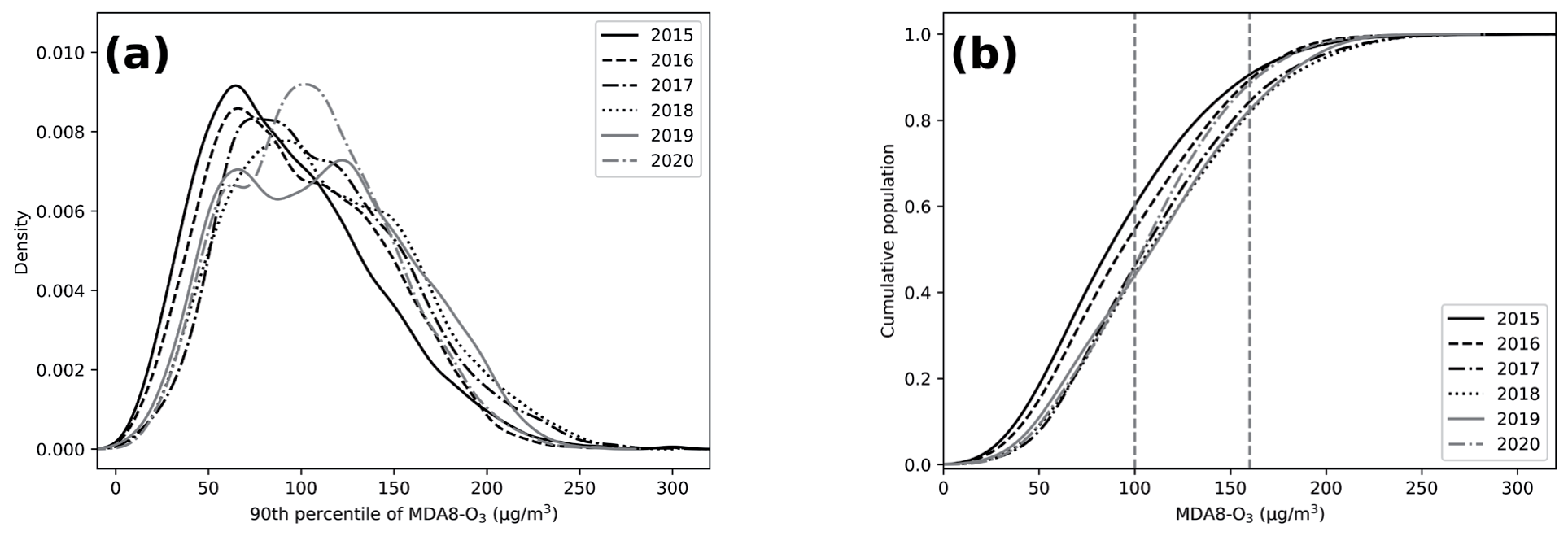
China’s Ambient Air Quality Standards (AAQS) set the following limits for the 8-hour average concentration of ozone, i.e., the primary standard (100 ug/m³) and the secondary standard (160 ug/m³). Fig. 2 shows the kernel density estimates and exceedance rates of O3 concentrations in the HREB from 2015 to 2020. Overall, the annual average O3 concentration in the HREB (90th percentile of MDA8-O3) gradually increased from 2015, then showed a slight downward trend in 2019 and 2020. O3 pollution remained a serious problem in the HREB. Specifically, the annual average O3 concentration in 2018 was 179.0 μg/m3, an increase of 14.0% compared to 2015 (157.0 μg/m3). Compared to 2018, O3 concentrations in 2019 (178.0 µg/m3) and 2020 (163.0 µg/m3) decreased by 0.6% and 8.4%, respectively. The State Council of the People’s Republic of China published the “Three-Year Action Plan for Winning the Blue Sky Defense War” (Plan) in June 2018. The Plan proposes that governments set stringent emission standards for industrial enterprises, in addition to strengthening the control of motor vehicle exhaust. According to previous studies [30], O3 concentrations in some major cities in China showed a downward trend from the 2019 year [27]. A decreasing trend in O3 concentrations in the HREB from 2019 was also found in this study, indicating that O3 pollution control measures worked.
As displayed in Fig. 2a), the kernel density curves of O3 concentrations were single-peaked in all years except for 2019, which is double-peaked. The change in the kernel density curve over time showed a shift to the right in the center as well as in the interval of change, with a small expansion in width. The height of the main peak of the kernel density curve showed a decreasing trend before 2019, followed by an increasing trend, which suggested O3 pollution has been reduced. The persistent increase in O3 pollution concentrations from 2015 to 2018 was largely caused by anthropogenic factors such as the increasing motor vehicle and petrochemical industries in China [30]. The kernel density curve in 2019 exhibited a double peak, and both peaks were reduced. Overall, O3 concentration decreased in 2019. This suggests that the Plan has been effective in the HREB. O3 concentrations displayed a significant increase in 2020. The lockdown during the COVID-19 epidemic in 2020 reduced anthropogenic emissions, resulting in a decrease in PM2.5 concentration. The decrease in PM2.5 concentration enhances solar radiation, leading to an increase in O3 concentration [14]. The proportions of MAD8-O3 exceeded the Chinese National Ambient Air Quality Standard I (CAAQS Class I; 100 μg/m3) in the HREB were 39.4%, 45.0%, 53.2%, 55.3%, 55.7%, and 58.9% from 2015 to 2020, respectively (Fig. 2b). This indicated that the increase in O3 concentration in the HREB slowed down, but O3 pollution is still relatively serious.
Monthly Variation
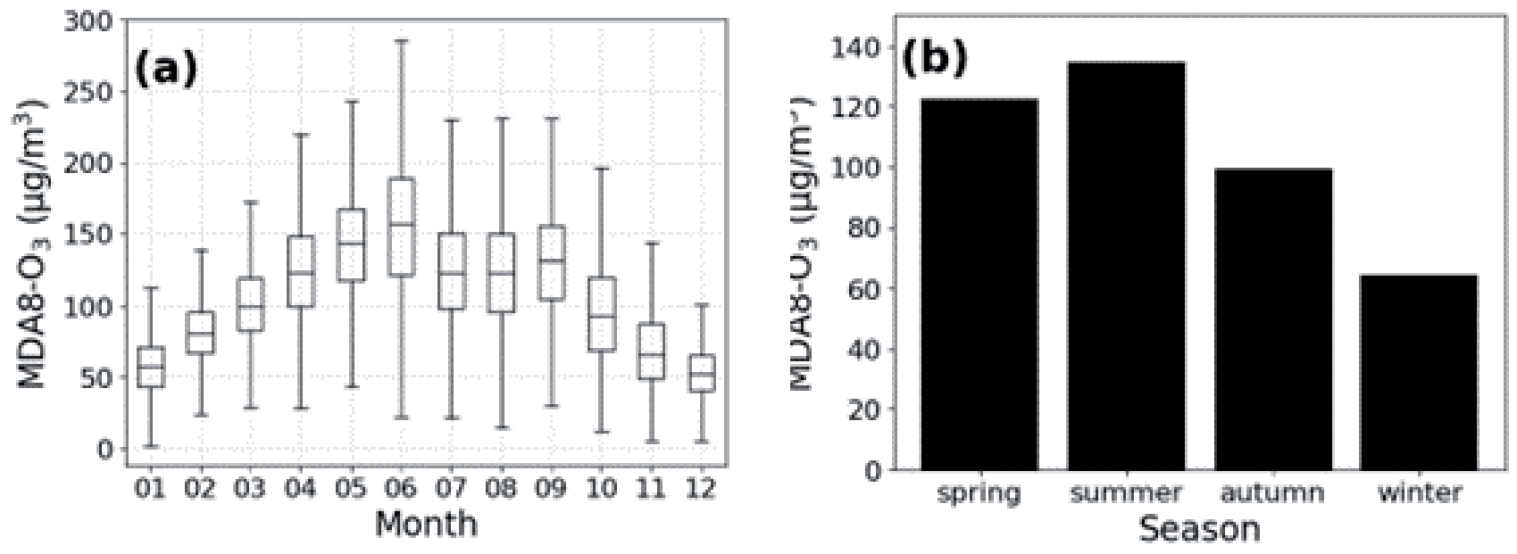
The monthly O3 concentration displayed an M-shaped bimodal variation with peaks in June, (155.3 μg/m3) and September (131.0 μg/m3) (Fig. 3a). It was found that the monthly O3 variation was related to the latitude in China, with a single-peaked structure usually found at latitudes above 35°N, while in most cases, a double-peaked structure is found south of 35°N [22, 40]. The latitude of the HREB is 31.7°N-35.4°N, and the bimodal structure of the O3 monthly variation in the study was the same as the results of previous studies. As shown in Fig. 3b, the seasonal averages of O3 concentrations in the HREB in spring, summer, autumn, and winter from 2015 to 2020 were 122.3, 134.7, 99.1, and 64.4 μg/m3, respectively. The O3 concentrations in the HREB demonstrated a characteristic of “high in spring and summer, low in autumn and winter”, which was consistent with the overall seasonal trend of O3 in East Asia. In summer, relatively high temperatures and intense radiation enhance photochemical reactions, which lead to increased O3 production [34].
Diurnal Variation
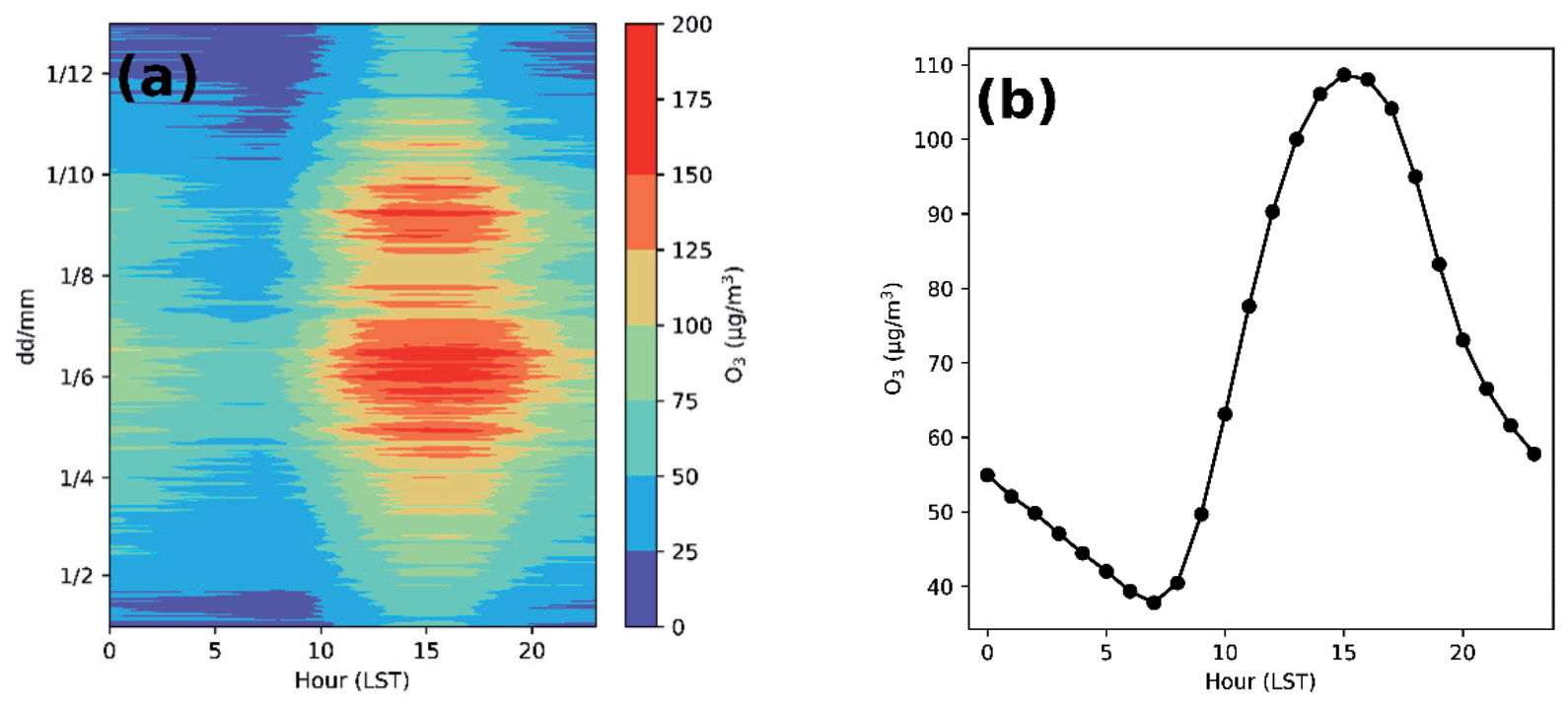
The diurnal variation of O3 concentration displayed a single-peak characteristic in the HREB (Fig. 4), with high levels during the day and low levels at night. As shown in Fig. 4a), O3 concentrations remained high at 20:00 (LT) during May-July. In June, O3 concentrations above 150 μg/m3 lasted for about 10 hours per day. During the daytime, with the rising sun and enhanced solar radiation, precursors such as VOCs and NOx participate in photochemical reactions and contribute to the formation of O3. As shown in Fig. 4b), the daily O3 maximum occurred at 15:00 (108.7 μg/m3) and the minimum at 7:00 (37.8 μg/m3). O3 concentration increased from 7:00 and decreased from 15:00. At night, the NOx titration reaction decreased the O3 concentration [41]. The time when the daily minimum and maximum O3 concentrations occurred was 1 hour after the average sunrise time and the average daily maximum temperature time, respectively.
Spatial Variations in O3 in the HREB
Standard Deviational Ellipse
The general changes in O3 spatial pattern in the HREB in different years were characterized by SDE analysis. As shown in Fig. 5, the annual O3 concentrations were mainly distributed in the southwest-northeast direction of the HREB. The azimuth of the ellipse increased from 84.10° in 2015 to 85.12° in 2018 and then decreased to 84.66° in 2020 (Table 1). Most developed cities in China are in the eastern coastal areas, and high O3 levels are usually found in those cities. The direction of movement of the ellipse was first to the southeast and then to the northwest (Fig. 5), which suggested the difference in O3 concentration between inland and coastal cities was decreasing. The mean center detected by SDE in the HREB was in southeastern Shangqiu. From 2015 to 2018, the center moved from 33.89°N, 116.40°E, to 33.80°N, 116.33°E, which indicated a greater decrease in O3 concentration in the northwestern part of the HREB. From 2018 to 2020, the center of O3 concentration in the HREB shifted from 33.80°N, 116.33°E, to 33.82°N, 116.36°E, which suggested a greater decrease in O3 concentration in the southwestern part of the HREB. The decrease in O3 concentration in the HREB mainly occurred in its western inland cities, which was similar to the O3 variations on a national scale [7]. The long axis of the ellipse decreased from 284.77 km in 2015 to 271.23 km in 2018, following a small increase in 2019 and 2020. The change in the long axis illustrated the spatial aggregation trend and spatial variation of O3 concentrations from 2015 to 2020. The ratio between the long and short axes of the ellipse showed a decreasing trend from 2015 to 2018, indicating a weakening trend of the directional distribution. Then the ratio increased in 2019 and decreased in 2020. In 2020, due to the influence of COVID-19, anthropogenic activities reduced remarkably, causing a decrease in the variability of O3 pollution among cities.
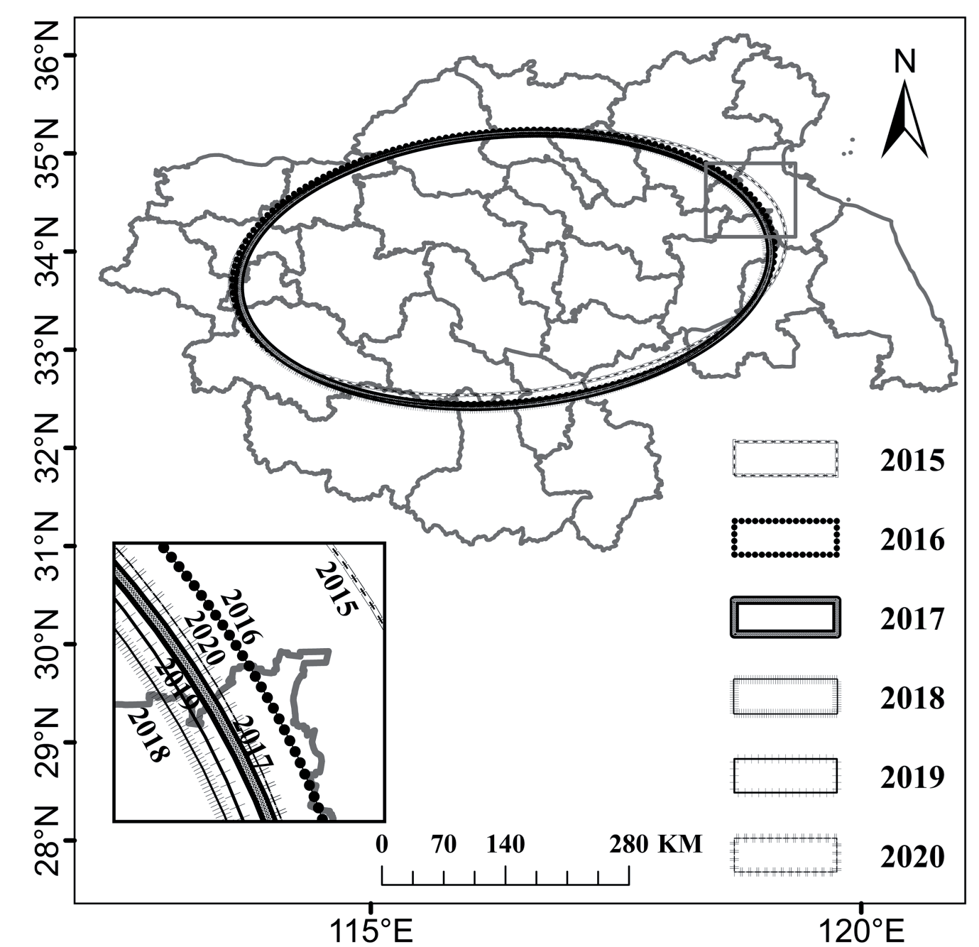
Table 1.
Parameters of the standard deviation ellipse in the Huaihe River Economic Belt (HREB).
Spatial Autocorrelation of O3 Concentrations
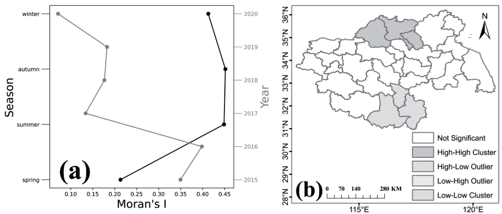
Global Moran’s I was calculated for different years and seasons in the HREB to discuss the spatial correlation of O3. From 2015 to 2020, the annual Moran’s I was 0.35, 0.40, 0.13, 0.18, 0.18, and 0.07, respectively. The seasonal Moran’s I was 0.21, 0.45, 0.45, and 0.41, respectively. The positive Moran’s I indicates positive spatial autocorrelation and spatial aggregation of O3 concentrations in the HREB, which suggests that O3 in cities may be influenced by their neighboring cities. The highest global Moran’s I in the HREB was found in autumn (0.452), followed by summer (0.449), indicating an enhanced aggregation of O3 concentrations. Therefore, it is necessary to carry out cross-city cooperation to control O3 pollution.
To identify the distribution and aggregation patterns of O3 pollution in cities in the HREB, a local spatial autocorrelation analysis was employed in this study. As shown in Fig. 6b), the most polluted cities were distributed in the northern part of the HREB, forming a high-high (HH) type of O3 concentration. Cities with HH concentrations included Heze, Jining, and Zaozhuang. These cities are located north of the HREB, having less precipitation and high energy consumption. Most of the surrounding cities are industrial cities with intensive anthropogenic emissions. The southern cities in the HREB have low O3 concentrations and have formed a low-low (LL) type. Cities with LL concentrations include Huainan, Luan, and Hefei. These cities are in the southern part of the HREB with abundant precipitation, which reduces O3 production. In conclusion, the agglomerated O3 pollution needs to be managed by joint efforts among cities, and more stringent measures should be taken in the northern part of the HREB.
Meteorological Driving Force
The correlation between individual meteorological factors and O3 concentration is listed in Table 2. O3 concentration showed a positive correlation with T and SSD in each city. This result is the same as that of the previous study [33]. The surface O3 is mainly generated by precursors through photochemical reactions, so O3 is sensitive to temperature and solar radiation [30]. Except for a positive correlation with RH in Rizhao, O3 concentration showed negative correlations with P, RH, and Pre in each city, among which the correlation with Pre in Rizhao and Zhengzhou was not significant. Rizhao is located east of the Yellow Sea and has a temperate monsoon climate with high precipitation and a humid climate. It is presumed that the correlation is not significant due to the prevalence of Pre and RH. Zhengzhou has a temperate continental climate with low precipitation, mainly concentrated in the summer, which caused a non-significant relationship between O3 concentration and Pre. The correlation of O3 vs. WS and O3 vs. WD was insignificant in all cities.
Table 2.
Correlation coefficients between O3 and meteorology for 27 cities in the HREB.
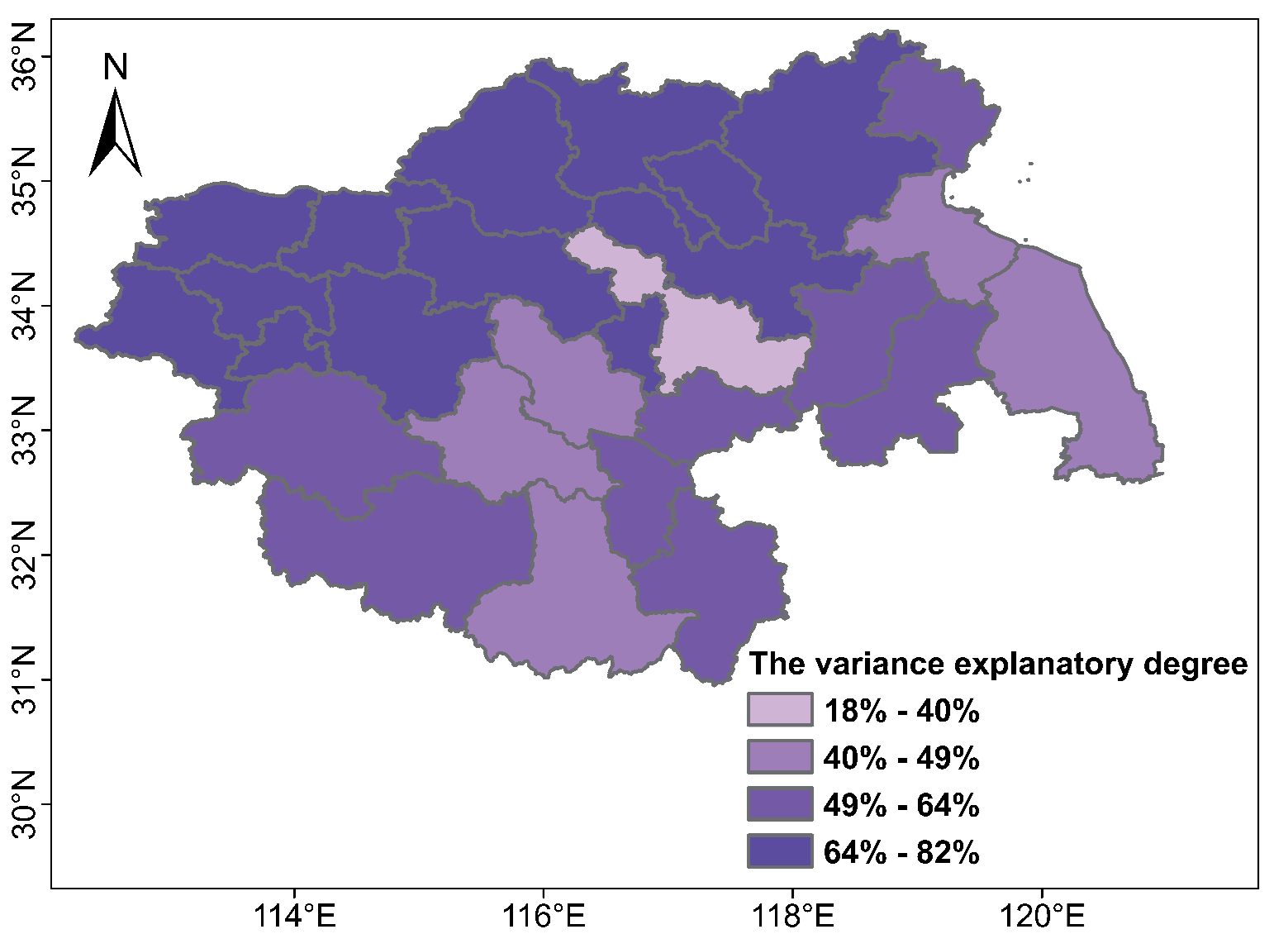
The MLR was used to determine the influence of meteorological conditions on O3 concentration in each city in the HREB from 2015 to 2020. The variance explanation rate reflects the influence of meteorological factors on O3 concentrations, with a value greater than 50.0% indicating a significant impact. Overall, meteorological factors can explain 82.2%~18.2% (60.5% on average) of the variation in O3 concentrations in the HREB. There were 21 cities with a variance explanation rate greater than 50%, accounting for 77.8% of all cities in the HREB. Cities with an explanation rate greater than 65.0% were concentrated in the northern part of the HREB. Specifically, Heze had the highest value (0.82). In Bozhou, Luan, Suizhou, Yancheng, Lianyungang, and Fuyang, meteorological factors have a relatively weak impact on O3 changes. In the northern part of the HREB, many industries are discharging massive anthropogenic pollutants [42]. Further, the northern part of the HREB is relatively flat and susceptible to monsoon winds [43]. These reasons all contributed to the high O3 concentration in the northern HREB. It is necessary to consider the specific influence of meteorological factors in different seasons in developing O3 pollution control measures.
Conclusion
In this study, the spatiotemporal distributions of O3 and the meteorological driving forces on O3 in the HREB were investigated using various interdisciplinary methods such as geographic analysis and spatial statistics. The results revealed that the annual average by 8.9% in 2020 (163.0 μg/m3) compared to 2018. O pollution remained an urgent issue in the HREB. The O3 concentration showed a bimodal variation with month, with the highest level in June (155.3 μg/m3). In season, O3 concentrations in the HREB displayed a characteristic of being high in spring and summer and low in autumn and winter. The daily variation of O3 increased during the day and decreased at night. The maximum daily O3 concentration occurred at 15:00 (LT) and the minimum at 7:00. In terms of spatial distribution, O3 concentrations in the HREB were mainly distributed in the southwest-northeast direction. SDE detected that the center of O3 concentration was in southeastern Shangqiu (33.80°N-33.89°N, 116.33°E-116.40°E). From 2015 to 2020, the center first moved southeast and then northwest. O3 concentration in the HREB showed positive spatial autocorrelation. The strongest spatial autocorrelation was found in the autumn. The most polluted cities were distributed in the northern HREB, including Heze, Jining, and Zaozhuang, forming a high-high (HH) aggregation. The cities in the southern HREB, including Huainan, Luan, and Hefei, have low O3 concentrations and have formed low-low (LL) clustering. O3 was positively correlated with T and SSD and negatively correlated with P, RH, and Pre in most cities. Meteorological factors can explain 82.2%~18.2% (60.5% on average) of the variation in O3 concentrations in the HREB. The O3 in the northern HREB was more affected by meteorological conditions than in the southern HREB.