Construction of an Indicator System to Assess SAD Level

Building on the theoretical foundations of Sustainable Agricultural Development (SAD), this article develops an indicator system that assesses SAD levels in terms of Resource Conservation, Environmental Friendliness, and Production Efficiency. Resource Conservation is reflected in the protection and rational utilization of all kinds of resources in the process of agricultural production, improving resource utilization efficiency to reduce natural resource consumption. Four specific indicators are chosen, namely the water-saving irrigation rate, the cropland replanting rate, the intensity of agricultural electricity consumption, and the level of fiscal support for agriculture. Environmental Friendliness refers to reducing pollution levels in agricultural production for the ecological environment (including greenhouse gas emissions from agricultural production). Select six specific indicators, including fertilization intensity, pesticide usage, agricultural membrane usage, agricultural Chemical Oxygen Demand (COD) emissions, agricultural ammonia nitrogen emissions, and the crop disaster rate. Production Efficiency refers to the comprehensive improvement of economic, ecological, and social benefits. Six specific indicators are identified, encompassing unit grain sowing area yield, unit agricultural machinery power output value, labor productivity, land output rate, the structural composition of the agricultural industry, and the degree of industry integration.

Using the Panel Entropy Weighting Method to Weight the Indicators

The Shannon Entropy Weighting method is an objective technique used to assign weights to indicators based on the magnitude of their information entropy. In addition, panel data can offer additional insights into the dynamic behavior of the samples. When exploring the development of SAD, it is also crucial to investigate how SAD has evolved over time in response to various factors in different provinces. Consequently, the panel entropy method is used in this article as a weight indicator.

Table 1 shows various indicators and weights. The indicator attribute “positive” means the value increases with the indicator data; “negative” means the value decreases with the indicator data. According to the weights and values of indicators, the evaluation value y of SAD in the 31 provinces (excluding Hong Kong, Taiwan, and Macao) from 2013 to 2021 can be calculated.

Using Kernel Density Estimation (KDE) to Explore the Evolution of SAD

We used the KDE method to fit the level of SAD in the 31 provinces from 2013 to 2021 to further explore its temporal evolution [25]. KDE is a non-parametric data distribution detection model that fits the distribution properties of the data [26]. As a statistical inference method based on data samples, Kernel Density Estimation does not need to make too many assumptions about the population distribution, so it can better reflect the actual situation of the data. The model form is as follows

where N = 31 is the sample size, y_i is the level of SAD in the i-th province, K(∙) is kernel function, h is density estimation bandwidth. Given that the Epanechnikov Kernel is optimal in terms of minimizing mean square error when determining the optimal bandwidth, and considering its minimal efficiency loss, this study selects the Epanechnikov Kernel as the kernel function, as outlined below.

Exploring the Agglomeration Effect of the Spatial Autocorrelation Model

Spatial Autocorrelation analysis enables the identification of spatial correlation patterns in the Sustainable Agricultural Development (SAD) levels across the 31 provinces examined in this study. The Global Moran’s I is employed to assess the presence of spatial clustering phenomena, and its calculation formula is provided below.

where w_ij is the adjacency weight of the i-th and j-th provinces. If the i-th and j-th provinces are adjacent, then w_ij = 1, otherwise w_ij = 0. To meet the needs of the model, Hainan and Guangdong are defined as adjacent and specifies w_ij = 0, if i = j.

The null hypothesis can be rejected, as the significant p-value suggests that the feature is not randomly distributed in the study area. At this stage, Local Moran’s I can be applied to identify the location, extent, and significance of agglomeration, and its calculation formula is provided below.

If I_i > 0, represents the spatial pattern of high-level provinces gathering to form a high-high agglomeration zone or low-level provinces gathering to form a low-low agglomeration zone; Conversely, I_i < 0 reflects the formation of high-low or low-high patterns, where high-level and low-level provinces interact.

Constructing a GTWR Model to Explore the Driving Factors of Agricultural Sustainability

The degree of SAD varies amongst provinces due to variations in their natural environments, geographic locations, and socioeconomic developments. This paper begins by examining the relationship between humans and the environment and selects five indicators, including Economic Development Level, R&D Investment, Human Capital Education, Agricultural Socialized Services, and Openness Levels. Table 2 shows driving factors and selected indicators. The specific instructions are outlined below.

(1) Economic Development Level.

Areas with high levels of economic development have a relatively high input-output ratio for agricultural production, which is strong in favor of promoting SAD.

(2) R&D Investment.

Technological advancements are pivotal in driving agricultural progress, with R&D investment fostering innovation in agricultural technologies and promoting the sustainability of agricultural development [28].

(3) Human Capital Education.

Human Capital Education has been shown to increase the innovation and flexibility of agricultural producers [29], leading to improvements in the efficiency and quality of agricultural production. This also enhances the competitiveness and resilience of the agricultural sector.

(4) Agricultural Socialized Services.

By providing professional,scientific and efficient services, agricultural socialized service organizations play a crucial role in enhancing various aspects of agricultural supply,including guarantee capabilities, technological innovation capabilities, sustainable development capabilities and international competitiveness. These services facilitate the adoption of sustainable agricultural technologies by smallholders, thereby transitioning conventional agriculture towards sustainable practices [30].

(5) Openness Level.

Advancing the comprehensive internationalization of agricultural practices is crucial for mitigating domestic resource shortages, alleviating resource and environmental pressures, and fostering a conducive environment for Sustainable Agricultural Development (SAD)[31].

This paper uses the GTWR model to explore the impact of these driving factors on SAD. The GTWR model is a regression linear model that periphrastically reflects the spatiotemporal heterogeneity characteristics of the study data by calculating the trends for changes in parameters with time and space [32, 33]. Currently, this method is predominantly applied in analyzing the scale and intensity of carbon emissions, rural settlement patterns, urban planning, and the spread of epidemics. It is less applied to the field of influencing factors in agricultural development, especially the driving factors of sustainable agricultural development. This paper uses the spatiotemporal and geographical weighted regression model to analyze the influence of various factors on agricultural sustainable development from the perspective of time and space and provides theoretical support and empirical experience for formulating relevant policies to promote agricultural sustainable development. The model is structured as follows.

where y_i is the SAD level of the i-th province, x_ik is the observed value of the k-th driving factor in the i-th province, (u_i, υ_i) is the spatial position coordinate of the i-th province, t_i represents the corresponding time dimension, β_k(u_i, υ_i, t_i) is the regression coefficient of the k-th driving factor in the i-th province, β₀(u_i, υ_i, t_i) is the spatiotemporal intercept of the i-th province, and ε_i represents the random error. If β_k > 0, then there is a positive correlation between the SAD and driving factors; otherwise, it is a negative correlation. The weighted least square method (WLS) is used to calibrate the GTWR model. The matrix expression of the estimated coefficients of the i-th province can be given as shown in formula (7).

Using the method of Huang et al. [33], the weight matrix is constructed based on adaptive bandwidth, Gaussian kernel function, and Euclidean distance.

Data Source and Processing

The data used in this study mainly comes from the China Statistical Yearbook, the China Statistical Yearbook on Environment, the China Agricultural Products Processing Yearbook, and the statistical yearbooks of provinces. Any missing data was completed using an interpolation method.

The Measurement Results of the SAD Level

This article used the panel Entropy Weight method to measure the evaluation index system of SAD [34] mentioned above and obtain the level values in 31 provinces in China from 2013 to 2021. Table 3 displays the results.

From a national perspective, the average level of SAD has been increasing year by year, from 0.326 in 2013 to 0.422 in 2021, with an average annual growth rate of 3.28%. This demonstrates China’s SAD is accelerating, and agriculture is transforming and upgrading. In addition, as can be seen from the measurement results, the level of SAD in China’s provinces from 2013 to 2021 showed significant spatial heterogeneity changes.

Based on a comparative analysis across provinces, Shanghai (0.546), Beijing (0.516), and Tianjin (0.487) rank highest amongst the provinces in terms of average sustainable agricultural development from 2013 to 2021. These three provinces have strong capacities for innovation in agricultural technology, high levels of economic development, and conditional advantages in SAD. The bottom three provinces are Xizang (0.234), Qinghai (0.251), and Yunnan (0.270). These three areas face limitations in terms of local agricultural resources and technological advancements, resulting in a relatively underdeveloped state of SAD.

The top three provinces are Hainan (7.776%), Guizhou (6.766%), and Zhejiang (5.86%) in terms of the growth rate of SAD levels; Jilin (-1.55%), Liaoning (0.04%), and Inner Mongolia (0.77%) are the lowest three provinces.

The Spatiotemporal Evolution of SAD

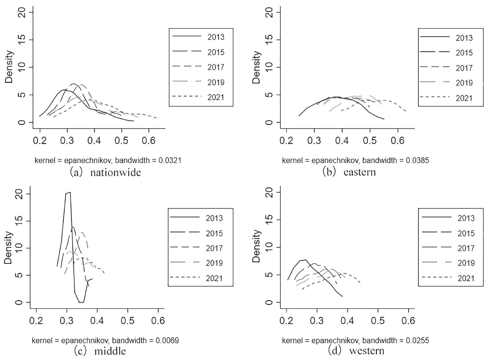
During the period of 2013 to 2021, the kernel density curves for SAD in different provinces, including the eastern, central, and western regions, all moved towards the right. This suggests that the level of SAD has progressively improved over time. There was a notable improvement in the degree of SAD in the eastern and western regions, as evidenced by the comparatively large changes observed in these regions, whereas the central region experienced relatively small changes (Fig. 1). The distribution pattern indicates that the primary peak of kernel density in the eastern region remains relatively stable, with an overall rightward shift in the estimated curve, indicating minimal internal variations within this region. However, in the central and western regions, there has been a consistent decrease in the main peak value of kernel density estimation each year, accompanied by an increase in bandwidth width. This suggests a widening gap in the levels of sustainable agricultural development among provinces in these regions. The maximum level of sustainable agricultural development at the national level experiences a rise followed by a decline, with the range of variation gradually expanding. The distribution shape indicates a “weak double peak” on the 2021 curve in the eastern region, but the difference in peak values is not statistically significant. Furthermore, the country’s overall curve displays a single peak and a gradually elongating right tail, suggesting that high-level provinces of SAD are emerging and the overall level of SAD is continuously improving.

Spatial Differentiation and Agglomeration Effect of SAD Level

Each province’s sustainable agricultural development level is categorized into four stages based on the maximum, minimum, and average levels of China’s SAD for each year: low level, medium-low level, medium-high level, and high level. A general improvement phenomenon of SAD was observed in different Chinese provinces between 2013 and 2021 (Fig. 2), and there was a significant overall spatial distribution heterogeneity, indicating a high level of development in the eastern coastal region and a low level in the western inland and northeastern regions. From the perspective of regional evolution types of SAD level, from 2013 to 2021, the proportion of low and medium-low level development cities gradually decreased from 38.71% in 2013 to 9.68% in 2021, and SAD in coastal provinces gradually entered a high level.

Fig. 1.

The spatiotemporal evolution of China’s sustainable agricultural development level.

Using Stata17 software to calculate the Global Moran’s I index from 2013 to 2021. The results are shown in Table 4.

The Moran index exhibited a p value below 0.05 across all years, indicating statistical significance. The results indicate a significant positive relationship between the level of SAD across various provinces in China. Moreover, the global Moran index has shown a consistent increase each year, indicating a strengthening agglomeration effect of these trends within each province over time. This shows that the nation has advocated ecological construction and sustainable development since the 12th Five Year Plan, and several provinces have stepped up their efforts to enhance SAD. The agglomeration effect has been strengthened by neighboring provinces’ experience with and borrowing from sustainable agricultural development initiatives.

Draw Local Moran’s I scatter plots for 2013, 2017, and 2021 (Fig. 3), with the four quadrants corresponding to four types in turn: high-high agglomeration zone, low-high agglomeration zone, low-low agglomeration zone, and high-low agglomeration zone. A high-high agglomeration zone refers to a region where both the province itself and its neighboring provinces exhibit high levels of sustainable agricultural development (SAD). Similar interpretations apply to other agglomeration patterns in different regions.

High-high agglomeration zones are primarily found in China’s eastern regions, which include Beijing, Tianjin, Jiangsu, Shanghai, and Zhejiang, as Fig. 3 illustrates. Guangdong and Hainan also displayed a high-high agglomeration situation in 2021. In the meantime, the high-high agglomeration zones progressively moved from the northeast to the southeast over time. Western China is the primary location for low-low agglomeration zones. These regions include Yunnan, Xizang, Ningxia, Gansu, Qinghai, Guizhou, and Shanxi. It’s evident that there is an obvious spatial agglomeration in SAD across different provinces, which is constrained by things like the natural geographic setting and the economic climate.

Analysis of Driving Factors for SAD

Analysis of Basic Regression Results

Based on the global linear regression model, using R4.2.2 software (RStudio) to estimate the coefficients. Table 5 demonstrates that the Economic Development Level, R&D Investment, Human Capital Education, Agricultural Socialized Services, and Openness Level exhibit a positive impact on SAD, aligning with the anticipated findings. Furthermore, all statistical tests conducted met the criteria for statistical significance at a 5% level. From the diagnostic information of the global regression model, if the variance inflation factor (VIF) of each explanatory variable is less than 7.5, it can be considered that there is no significant multicollinearity between the explanatory variables. At the same time, it was found that the determinability coefficient of the model was relatively high (R² = 0.8172), indicating a good fit of the global regression model and a strong explanatory power of the model.

Fig. 2.

The level and changes of sustainable agricultural development in various provinces of China in 2013, 2017, and 2021.

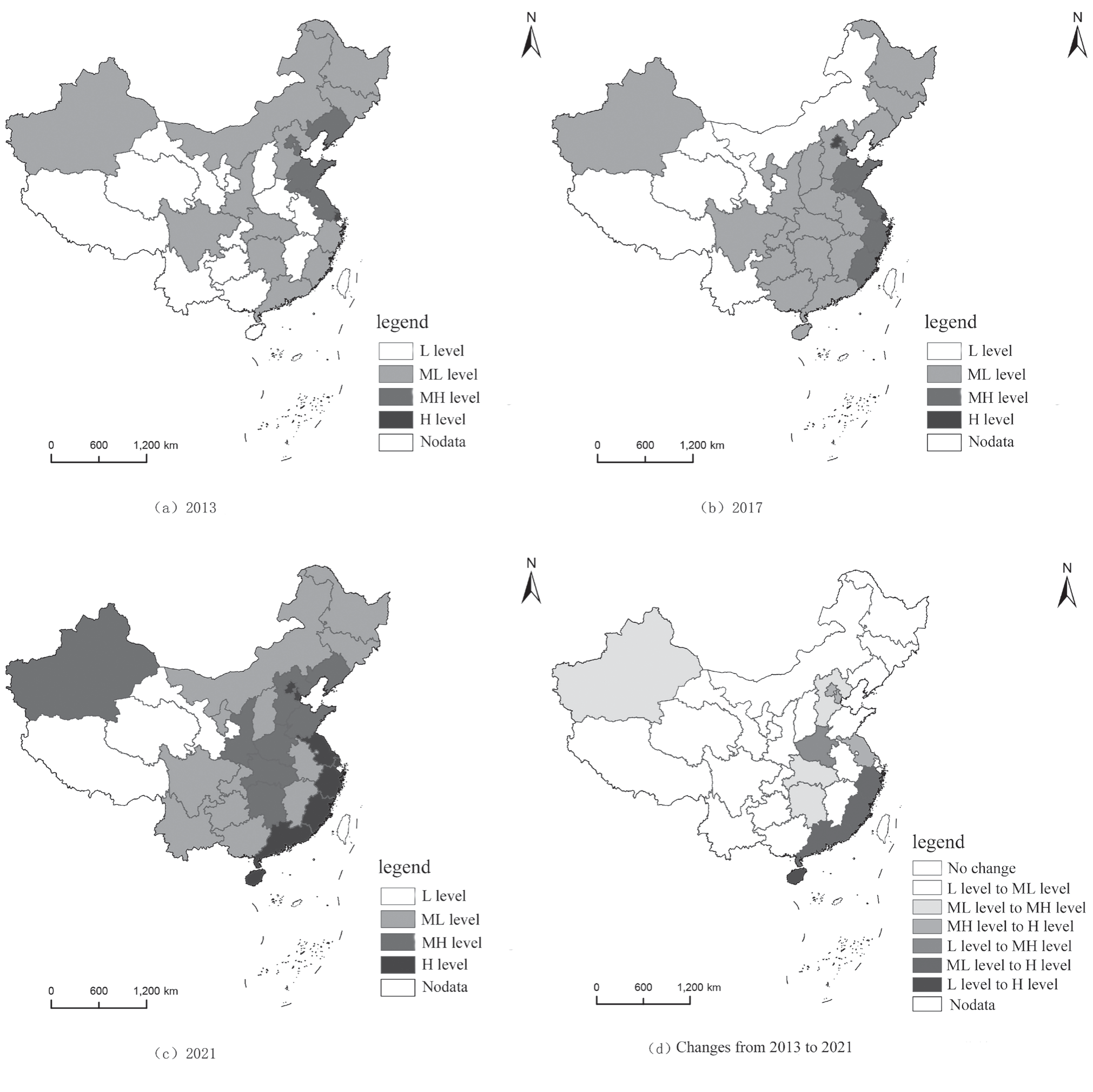
Table 4.

Global Moran’s I index of the level of sustainable development in agriculture.

Year	2013	2014	2015	2016	2017	2018	2019	2020	2021
Moran’s I	0.341***	0.376***	0.392***	0.429***	0.436***	0.452***	0.478***	0.475***	0.483***
Z	3.179	3.475	3.589	3.905	3.959	4.111	4.288	4.298	4.337
P-value	0.002	0.001	0.000	0.000	0.000	0.000	0.000	0.000	0.000

Fig. 3.

Scatter plot of the Moran Index for the overall level of sustainable agricultural development in various provinces across China in 2013, 2017, and 2021.

Fig. 4.

Time variation of GTWR regression coefficient from 2013 to 2021.

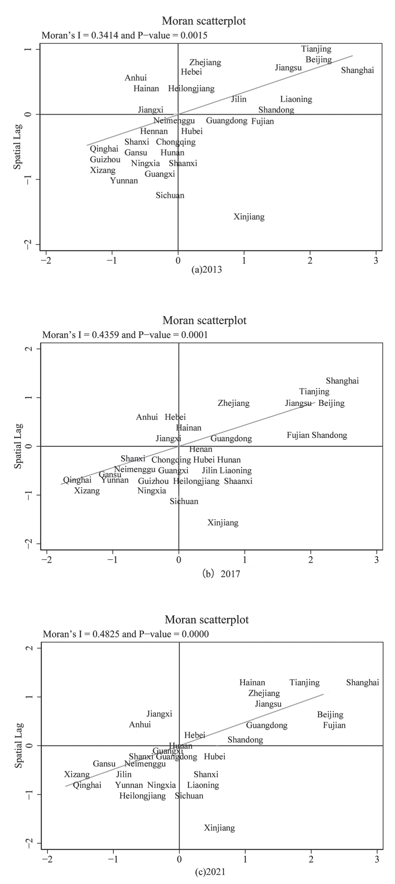
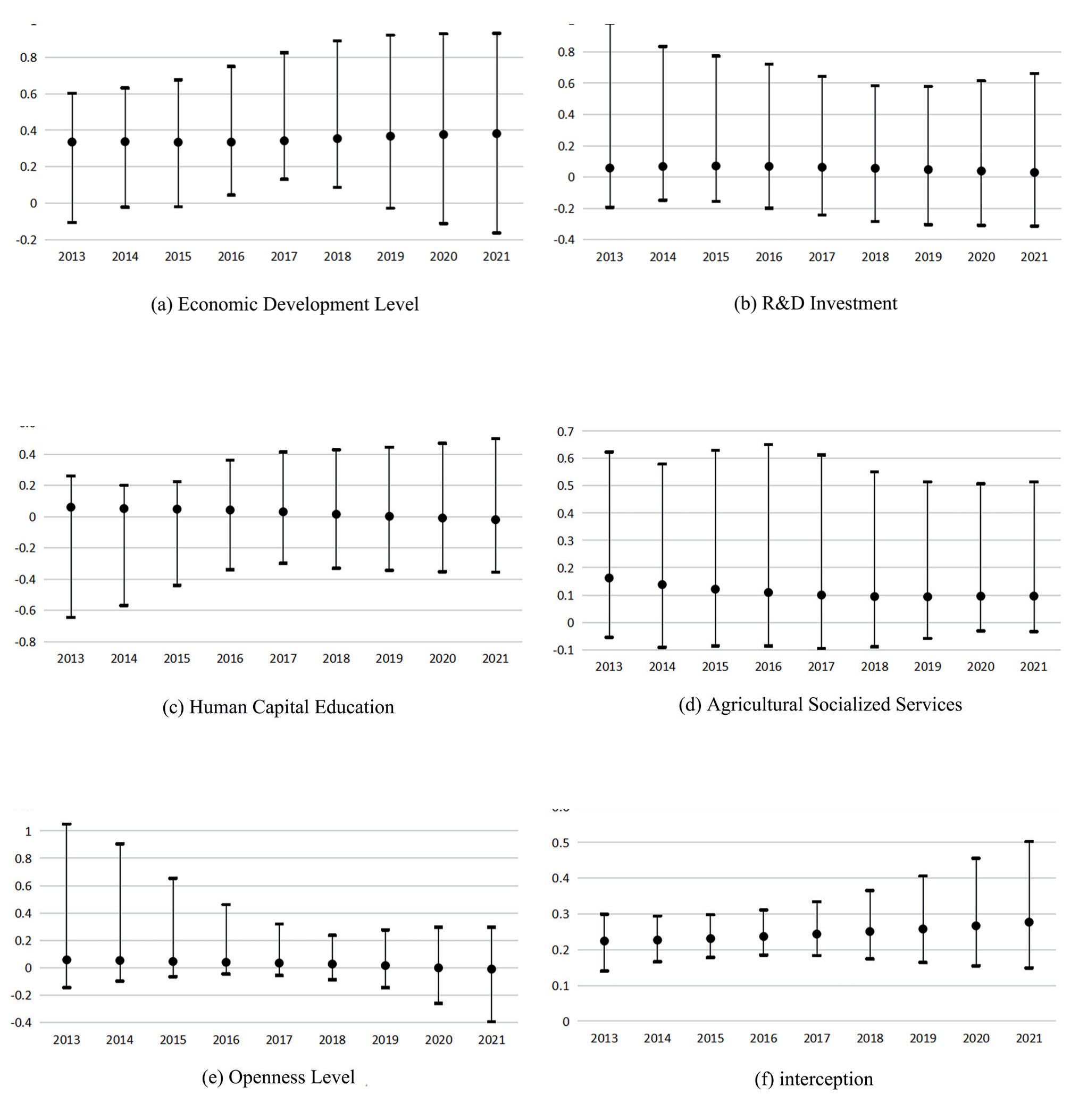
Table 5.

Basic linear regression results.

Factors	Estimate	Std. Error	t value	Pr(>|t|)	VIF
(Intercept)	0.237	0.005	46.701	< 2e-16 ***	—
Economic Development Level	0.335	0.016	21.265	< 2e-16 ***	1.671
R&D Investment	0.037	0.016	2.254	0.025 *	2.179
Human Capital Education	0.048	0.012	3.905	0.000 ***	1.488
Agricultural Socialized Services	0.084	0.013	6.232	1.74e-09 ***	1.387
Openness Level	0.056	0.018	3.041	0.003 **	1.536

The Influence of Driving Factors Presents Spatial Heterogeneity

This study visualizes the regression coefficient intervals of each driving factor and investigates their spatial heterogeneity to intuitively describe the impact of various driving factors on SAD in various provinces. Using the natural breakpoint principle, we found the mean of the regression coefficients for each driving factor from 2013 to 2021, as indicated in Fig. 5.

The regression coefficient of the Economic Development Level from Fig. 5(a) demonstrates a trend of increasing from north to south. Economic Development in Guangdong, Guangxi, and Hainan provinces has a significant impact on SAD. This is attributed to the higher level of economic development in the southern region, where agricultural development initiated the green transformation earlier, providing substantial momentum for the sustainable development of agriculture. The northern and western regions are experiencing a slight slowdown in economic development, and there is little to no impact of this on SAD.

From Fig. 5(b), (c), and (d), we can observe that the regression coefficients for R&D Investment, Human Capital Education, and Agricultural Socialized Services all exhibit a consistent upward trend from the southeast to the northwest. This is due to the higher levels of R&D Investment, Human Capital Education, and Agricultural Socialized Services in the southeast, leading to a maturing and stabilizing impact on SAD. In contrast, the northwest is experiencing rapid growth in technology, human capital, and agricultural services for sustainable development in agriculture, resulting in a greater overall impact.

Fig. 5.

Regression coefficients of various driving factors from 2013 to 2021.

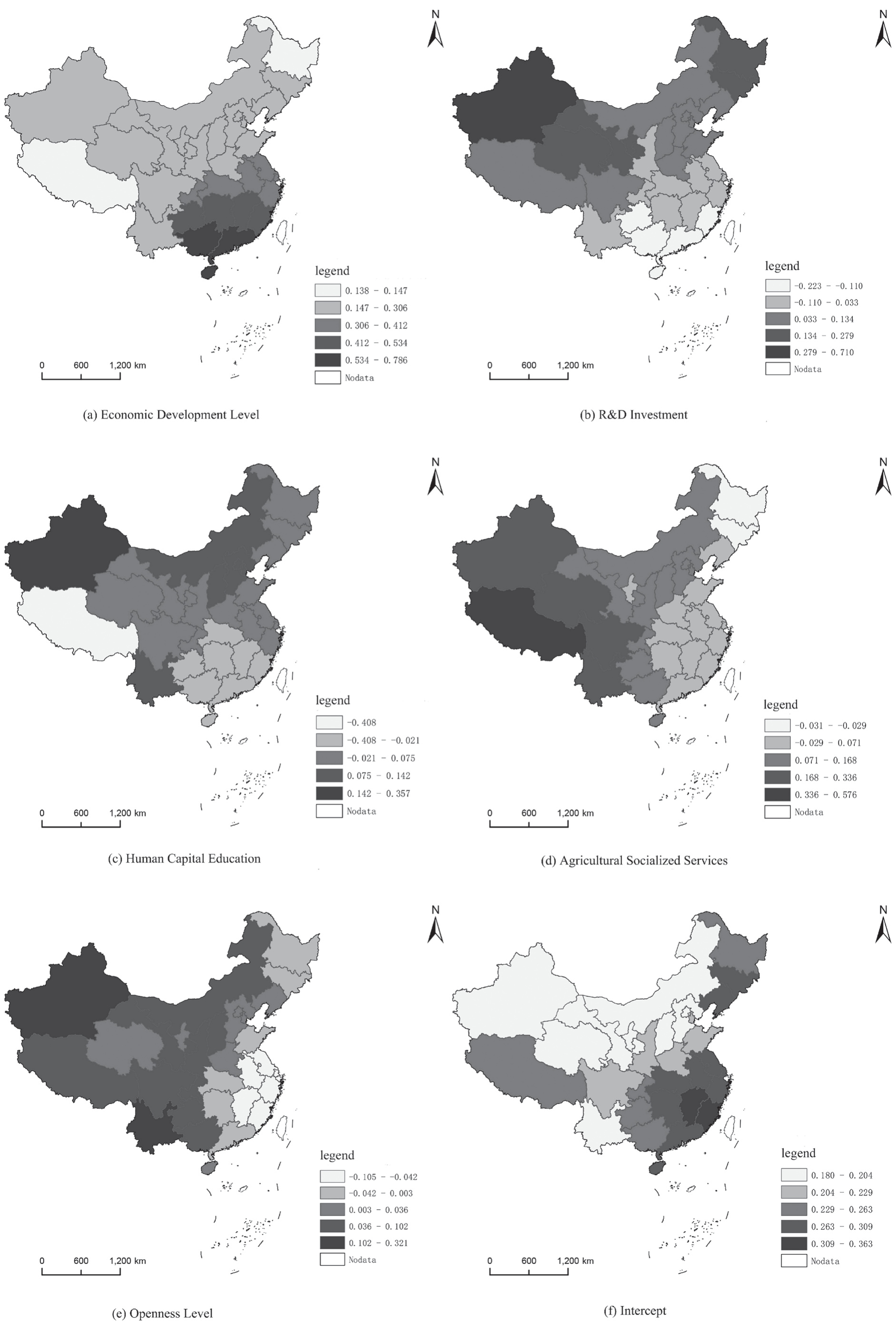
From Fig. 5(e), the regression coefficient of Openness Level shows an increasing trend from the eastern coastal areas to the western inland areas, indicating that Openness Level in the eastern coastal areas is relatively high. As the level of Sustainable Agricultural Development (SAD) continues to improve, its impact has gradually diminished. However, in recent years, with the persistent advancement of international trade initiatives such as the Belt and Road Initiative, the openness level of the western inland regions has progressively increased, resulting in a greater influence on SAD.

From the above analysis, the impact of various driving factors on the level of SAD shows spatial heterogeneity.