

Introduction
Terrestrial evapotranspiration (ET) comprises vegetation transpiration (Ec), soil evaporation (Es), and the interception of evaporation from the vegetation canopy (Ei). This is crucial for the water and carbon cycles and the soil-plant-atmosphere energy balance. ET can significantly influence climatic systems, surface hydrological processes, and biogeochemical cycling within terrestrial ecosystems [1-3]. Although the potential impacts of climate change on ET have been well explored, ET can be significantly affected by anthropogenic land use/land cover changes (LUCC) that can further influence the water resource allocation [4]. The anomalous ET states from climate change and land cover alterations can worsen the water supply-demand imbalance, impeding the global sustainable development efforts [5]. Therefore, accurately identifying spatiotemporal ET variations and studying the impacts of LUCC on ET dynamics are crucial for the allocation of water resources and the scientific management [6].
With recent advancements in remote sensing technology, the monitoring of terrestrial natural resources, particularly high-resolution ET observations, has improved. Remote sensing-based ET models, including the Penman-Monteith (PM) [7], Priestley-Taylor (PT-JPL) [8], Surface Energy Balance System (SEBS) [9], and Hybrid Two-Source Energy Balance Model (HTEM) [10], are commonly applied for global-or regional-scale ET simulations [11]. The Priestley-Taylor method is especially noteworthy for its simple yet effective approach to estimating the potential ET from saturated surfaces, eliminating the need to parametrize canopy and aerodynamic resistances, as in PM-type methods. Fisher et al. (2008) [12] developed a multi-constraint biophysical framework to convert potential ET into actual ET according to this method, leading to the PT-JPL model, a simple remote-sensing-based ET model. It presented a clear physical interpretation and minimal requirements for forcing the data. It included vegetation variables, including the Fraction of Intercepted Photosynthetically Active Radiation (FIPAR), Fraction of Absorbed Photosynthetically Active Radiation (FAPAR), and Leaf Area Index (LAI), which can be estimated using empirical equations based on the Normalized Difference Vegetation Index (NDVI). These were globally applicable and exhibited good accuracies. However, the quality of the original input imagery could significantly affect the accuracy of the ET retrieval. Despite their short revisit periods, high temporal resolution remote sensing data may lack the spatial resolution required for extensive and heterogeneous surface ET studies. Conversely, remote sensing data with high spatial resolution, which can capture detailed spatial ET patterns, often have longer revisit periods and potential image gaps. In practical research, it is vital to achieve a balance between high temporal and spatial resolutions in remote sensing imagery. Various methods aided by multisource remote sensing data fusion techniques have emerged to address inherent temporal and spatial discrepancies in remote sensing data [13]. Recent applications of data fusion methods for optimizing ET inversion can be broadly categorized into two types: (1) the fusion of high spatiotemporal resolution land surface temperature datasets and reflectance images as inputs for ET model parameters [14] and (2) the fusion of multiscale ET products derived from remote sensing data with high spatial and temporal resolutions [15]. For instance, Chen et al. [16] proposed a time series reconstruction approach, termed gap-filled with Savitzky-Golay (GF-SG), using the Google Earth Engine (GEE) platform. This method combines gap filling with SG filtering, offering effective interpolation and prediction for data with long periods of missing values. In addition, it performed well in identifying and interpolating cloud detection errors while conserving local computational resources through its implementation on GEE.
The NDVI time series was reconstructed by initially employing the GF-SG model for the Yellow River Basin of Inner Mongolia. The 8-day 30m NDVI time series data were then used as input for the PT-JPL model for enhancing the spatiotemporal resolution of ET. The model sensitivity parameters were optimized using land use dynamic data and eddy covariance observation site data to enhance ET simulation accuracy. Subsequently, the spatiotemporal characteristics of ET within the basin were analyzed, and the impacts of land use transfer on ET changes were examined. The objectives were: (1) to interpret the ET in the specified research area from 2000 to 2022 using the PT-JPL model with high precision; (2) to identify the spatiotemporal characteristics of ET from 2000 to 2022; and (3) to assess the impacts of land use dynamic transfer on evapotranspiration within the basin over 23 years. This study could offer valuable insights into water resource management that may improve the efficiency of water resource utilization.
Overview of the Research Area
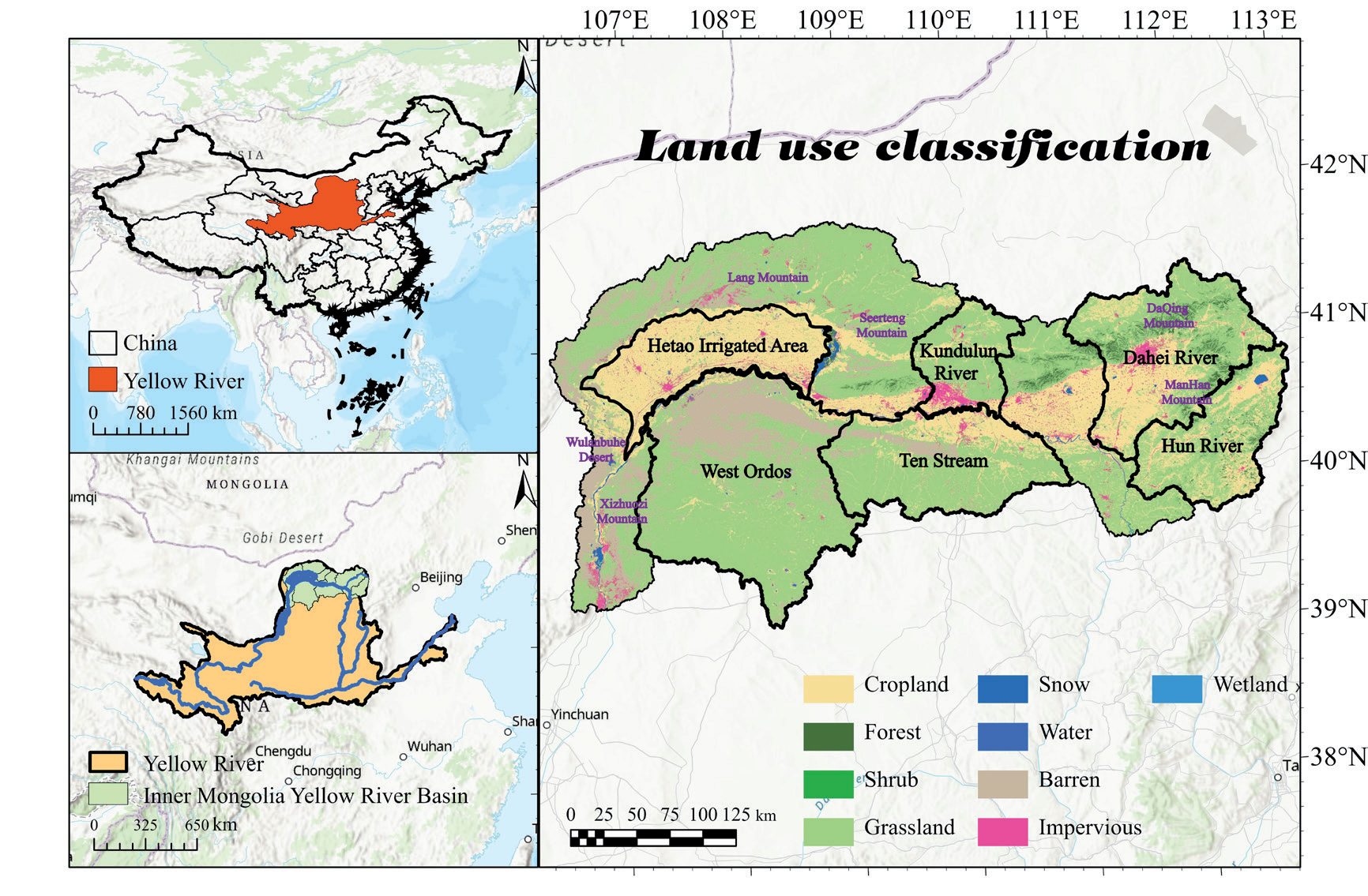
The Yellow River Basin in Inner Mongolia spans 830 km, starting from Shizuishan City, Ningxia, and passes through five leagues, Wuhai, Bayannur, Ordos, Baotou, and Hohhot, before exiting Zuoqi. The basin, covering approximately 105,000 km² with elevations ranging from 1000 to 1500 m (Fig. 1), features a landscape of hills, forests, farmland, grassland, deserts, rivers, lakes, and other landforms. This includes the Hetao Irrigation District, where crops are the main component, the Daqing Mountains area with higher forest cover, and the Ulan Buh and desert regions characterized by low vegetation cover due to arid climate. The area falls within a semi-arid and arid temperate continental monsoon climate zone, known as dry and rainy springs, and long, harsh winters. The average annual temperatures are in the range between 2.04°C and 9.79°C, and the average annual precipitation is 297.25 mm.
Materials and Methods
Data and Processing
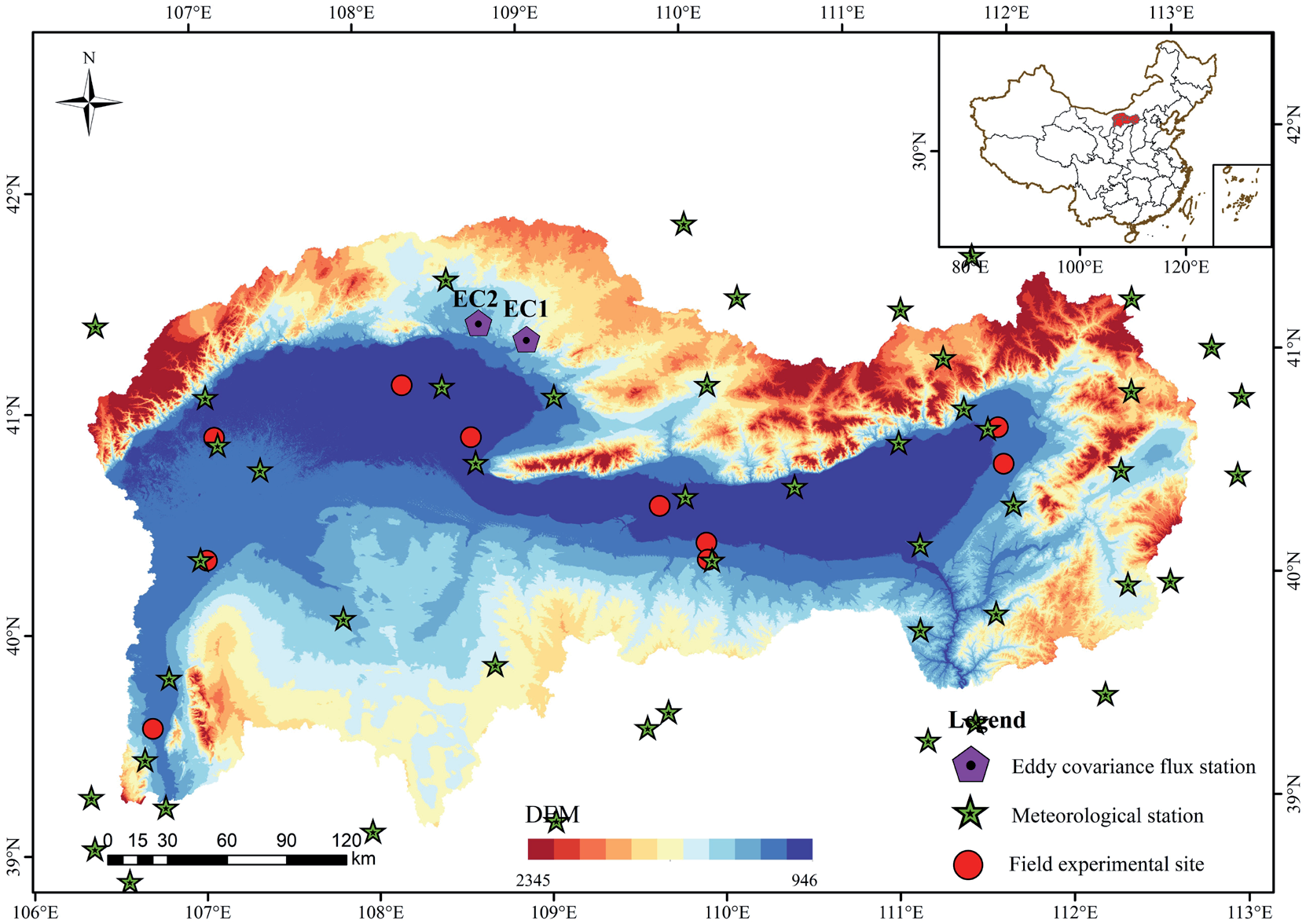
Daily surface meteorological data were provided by the China Meteorological Science Data Center (https:// data.cma.cn/; accessed August 10, 2023). We used the Chinese Surface Meteorological Dataset (V3.0), which included daily data for pressure, 0 cm soil temperature, sunshine hours, wind speed and direction, relative humidity, evaporation, precipitation, and temperature. These data were collected from 824 reference and basic meteorological stations in China in January 1951. Data, including pressure, temperature, and relative humidity, were collected from 50 meteorological stations in the research area for the years 2000–2022, including pressure, temperature, and relative humidity. Using Python's Kriging interpolation method, these variables were interpolated to a 30 m spatial resolution using the coordinates in the WGS 1984 coordinate system. The FAO Penman-Monteith formula was adopted to compute the net radiation data. The parameter calibration and validation of the PT-JPL model were conducted using data from two eddy covariance (EC) stations within the basin for the years 2015-2017 (EC1 and EC2), representing grassland and shrubland land cover types, respectively.
The MOD09A1 reflectance products from 2000 to 2022 were obtained from Google Earth Engine (https:// earthengine.google.com/, accessed on July 8, 2023). We derived 8-day 500 m NDVI data through cloud masking and spatial interpolation. Additionally, we calculated 16- day 30 m NDVI data from the Landsat 5, 7, and 8 bands. Vegetation Fractional Cover (FVC) data were estimated using a linear spectral unmixing model. Leaf Area Index (LAI) data were estimated using an empirical statistical model that incorporated coefficients as shown in Fig. 2 derived from field experiments.
The adopted land use dataset was the China Land Cover Dataset (CLCD) released by Wuhan University and provided by Xin Huang (https://zenodo.org/). This dataset spanned 1985 to 2022 at a 30 m spatial resolution, including nine land cover classes: wetland, impervious surface, bare land, ice/snow, water body, grassland, shrubland, forest, and cropland.
Research Methodology
GF-SG Model
Owing to the extended revisit period and susceptibility to cloud contamination associated with the Landsat satellite series, Landsat NDVI time series data often exhibit temporal discontinuity [17]. The gap-filling and Savitzky-Golay filtering (GF-SG) methods were applied to reconstruct high-quality Landsat NDVI time-series data. This approach integrated cloud-free Landsat observations and MODIS NDVI time series data to fill the missing values in the original Landsat NDVI time series data, generating synthetic 8-day 30m resolution NDVI time series data. Weighted Savitzky-Golay filters were used to eliminate the residual noise from the synthesized time series. This method involved two primary steps.
The GF-SG method was first applied to fill in the missing values in the original Landsat NDVI time-series data. Owing to potential discontinuities in the original data and the limited availability of cloud-free investigations over a one-year period, simple linear interpolation or curve fitting is ineffective for filling the missing values. MODIS NDVI images that exhibited high spatial autocorrelation were initially selected for the GF-SG model. The bicubic interpolation method (M_interpol) was utilized for spatially resampling the images to 30 m resolution through utilizing bicubic interpolation method (M_interpol). Subsequently, the correlation coefficient between the cloud-free Landsat observations and M_interpol was computed for the target pixel using the GF-SG. Based on this correlation coefficient, similar pixels within a local neighboring window (40 × 40 pixels, approximately 1.2 × 1.2 km2) were identified for each target pixel. The pixels with correlation coefficients higher than 0.8 were considered similar to the target pixel (denoted as M_similar_ series(xj, yj)). These pixels were used to generate synthetic NDVI time series data for the target pixel. The specific formula is as follows [18]:
where 𝑤(𝑥𝑗,𝑦𝑗) denotes the weight of the 𝑗𝑡ℎ similar pixel, and 𝑛n represents the number of similar pixels. Moreover, 𝑤(𝑥𝑗,𝑦𝑗) was determined based on the similarity between the target pixel and time series data of the jtℎ similar pixel, quantifying the similarity by calculating their correlation coefficient. To address the discrepancies in NDVI values between Landsat and MODIS data (e.g., caused by differences in spectral response functions), the GF-SG method integrated shape model fitting. It utilizes a linear transfer function to adjust Mreference(x,y):
In this process, 𝑎(𝑥,𝑦) and 𝑎0(𝑥,𝑦) are determined by minimizing the difference between the cloud-free Landsat observations of the target pixel and 𝑀𝑎𝑑𝑗𝑢𝑠𝑡𝑒𝑑(𝑥,𝑦). In the following step of the GF-SG, a weighted filter was applied to smooth the synthesized NDVI time series and reduce the residual noise. The weighting of the SG filter was based on the following two principles. First, the maximum weight was assigned to the initial cloud-free Landsat observations to preserve them optimally. Second, larger weights were assigned to filled NDVI values if spatial variations in NDVI images on certain dates within the synthesized NDVI time series were small and vice versa. This principle could be effective because of the greater reliability of spatial resampling for homogeneous landscapes. For more detailed information on the GF-SG method, please refer to Chen et al. [16].
PT-JPL Model
The PT-JPL model partitions ET into canopy transpiration (Ec), interception evaporation (Ei), and soil evaporation (Es), calculated as follows [19].
(1) Calculate the regional-scale net radiation data required for the model input.
where 𝑅𝑛 represents the surface net radiation (W/ m²); 𝑅𝑛𝑠ℎ𝑜𝑟𝑡 and 𝑅𝑛𝑙𝑜𝑛𝑔 represent the input net shortwave radiation and output net longwave radiation, respectively (W/m²); 𝐼𝑡 denotes the downward shortwave solar radiation (W/m²); 𝛼 stands for the surface albedo; 𝜎 is the Stefan-Boltzmann constant (5.67×10⁻⁸ W/(m2/K4)); 𝑅𝑙𝑢 is the upward longwave radiation (W/m²); 𝑅𝑙𝑑 is the downward longwave radiation (W/m²); and 𝑇 represents air temperature (K).
(2) Calculation of the net radiation components 𝑅𝑛𝑠 and 𝑅𝑛𝑐:
where 𝑅𝑛𝑠 represents the net radiation at the soil surface (W/m²), 𝑅𝑛𝑐 denotes the net radiation intercepted by the vegetation canopy (W/m²), 𝑘𝑅𝑛 stands for the extinction coefficient (0.6), and 𝐿𝐴𝐼 represents the leaf area index (m2/m-2).
(3) Calculation of each influencing factor
where 𝑅𝐻 denotes relative humidity (%), 𝑇 stands for air temperature (°C), 𝑉𝑃𝐷 represents vapor pressure deficit (kPa), 𝛽 indicates the sensitivity of soil moisture constraint to VPD (kPa), and 𝑇𝑜𝑝𝑡 is the optimum temperature for plant growth (°C). 𝑓𝑤𝑒𝑡 denotes the relative humidity constraint factor, 𝑓𝑔 represents the green canopy constraint factor, 𝑓𝑡 stands for the temperature constraint factor, 𝑓𝑀 denotes the moisture constraint factor, 𝑓𝑆𝑀 represents the soil moisture constraint factor, 𝑓𝐴𝑃𝐴𝑅𝑚𝑎𝑥 is the maximum 𝑓𝐴𝑃𝐴𝑅, 𝑓𝐴𝑃𝐴𝑅 is the fraction of PAR absorbed by the canopy (unitless), and 𝑓𝐼𝑃𝐴𝑅 is the fraction of photosynthetically active radiation (PAR) intercepted by the canopy (unitless). 𝑓𝐼𝑃𝐴𝑅 and 𝑓𝐴𝑃𝐴𝑅 are defined as follows:
where 𝑏1=1.2×(−0.04), 𝑏2=−0.05, 𝑘2=1, and 𝑘1 and 𝛽 are parameters to be optimized, with 0≤𝑘1≤1.4 and 0≤𝛽≤1 [20].
where Δ denotes the slope of temperature-saturation vapor pressure curve, 𝑒𝑎 represents actual vapor pressure (kPa), 𝑒𝑠 denotes saturation vapor pressure (kPa), and 𝑇𝑚𝑖𝑛 stands for minimum air temperature (K), taken as the minimum value of monthly average temperatures.
where 𝐹𝑉𝐶 denotes the fraction of vegetation cover, 𝐺 represents the soil heat flux, Γs is taken as 0.325 for low vegetation cover, and Γc is taken as 0.05 for high vegetation cover. 𝑁𝐷𝑉𝐼𝑚𝑖𝑛 is taken as 0.05, and 𝑁𝐷𝑉𝐼𝑚𝑎𝑥 is taken as 0.75.
(4) The equations for calculating evapotranspiration (ET) and its components are as follows.
where 𝐸𝑐 represents vegetation transpiration (W/ m²), 𝐸𝑠 denotes soil evaporation (W/m²), 𝐸𝑖 stands for interception evaporation by the vegetation canopy (W/ m²), 𝛼 represents the Priestley-Taylor coefficient, taken as 1.26, and 𝛾 represents the psychrometric constant (kPa/°C), taken as 0.066 [21].
The Mann-Kendall Test and the Theil-Sen Median Trend Analysis
The Mann-Kendall (M-K) test was combined with the Theil-Sen Median trend analysis to assess trends in the ET time series. This approach was robust against discrete data and measurement errors, without requiring sequence values to maintain a normal distribution during significance testing. In addition, it did not assume a linear trend without being affected by outliers or missing values. It has been widely used for the significant trend testing of long time-series data. The Theil-Sen trend analysis was a robust non-parametric computational method, formulated as [22]:
where β > 0 demonstrates an increasing trend in ET; conversely, β < 0 presents a decreasing trend in ET, and β = 0 suggests no change in trend. ETj and ETi represent the ET values for the jth and ith year, respectively.
Using the M-K test to assess the significance of ET trends, the calculation formula is as follows.
The test statistic was calculated as follows:
The sign function:
The standardized statistic:
where sgn represents the sign function, the statistical quantity Z ranges within (−∞, +∞), and n is the time-series length. At a given significance level α, |Z|>Z1-α/2 presents a significant change in the ET sequence at the α level. This study specified α = 0.05 as the confidence level to determine the significance of the ET time series trend.
Hurst Exponent Analysis
The Hurst exponent analysis quantitatively describes long-term dependence in time series data and has wide applications in hydrology, climatology, ecology, and other fields. This enables the prediction of future trends by analyzing past trend changes in long time-series data. Its basic principles are as follows [23]:
For a time series
The cumulative deviation:
The range:
The standard deviation:
If there exists
Land Cover Transfer Model
The land cover transition matrix is a two-dimensional matrix that can examine the relationship between land changes in the same area at different time sequences. It represents the inflow and outflow of land-use types from the initial to the final period and reveals the direction of land-use transfer. The mathematical form of the land use transfer matrix is as follows [24]:
where 𝑆𝑖𝑗 denotes the area conversion from land types 𝑖 to 𝑗 in time period 𝑛; 𝑖 and 𝑗 are the previous and subsequent land use types, respectively; and 𝑛 is the number of land use types within a period.
Model Evaluation Metrics
The prediction accuracy of the model was evaluated by adopting the coefficient of determination 𝑅2, the root mean square error (RMSE), the slope of the trend, the mean absolute error (MAE), and the intercept 𝑑 [25].
The formula for RMSE calculation is as follows:
where 𝑛 represents the number of samples, 𝑦𝑖 denotes the actual observed values, and pi represents the modeled or simulated values. A smaller RMSE value indicates a better model performance.
The degree of correlation between the model simulation results and actual observations was represented by the Pearson correlation coefficient (R), which ranged from 0 to 1. When 𝑅=1, it indicates a perfect linear relationship between the two datasets. The calculation can be performed using the following equation:
where Xi represents the actual test data, Yi denotes its mean value, Yi signifies the regional mean of the model simulation results, and Ȳ represents its mean value. A higher 𝑅 value suggests a more accurate simulation of the model's trend with respect to the observed data.
The temporal trends of various data elements were calculated using linear regression equations, with the trends represented by the slope of the regression line. The equation used was as follows:
where “slope” represents the temporal trend of water temperature vegetation elements; “n” is the length of the data's time series. A negative or positive value of the slope indicates a decreasing or increasing trend in the data.
The MAE accurately reflected the magnitude of the actual prediction errors. It assessed the deviation between the observed and fitted values, with a value closer to 0 indicating better model fitting and higher prediction accuracy. The equation used is as follows:
where Pi represents the simulated result, Yi represents the actual value, and 𝑛 denotes the sample number.
Results
Simulated NDVI Results
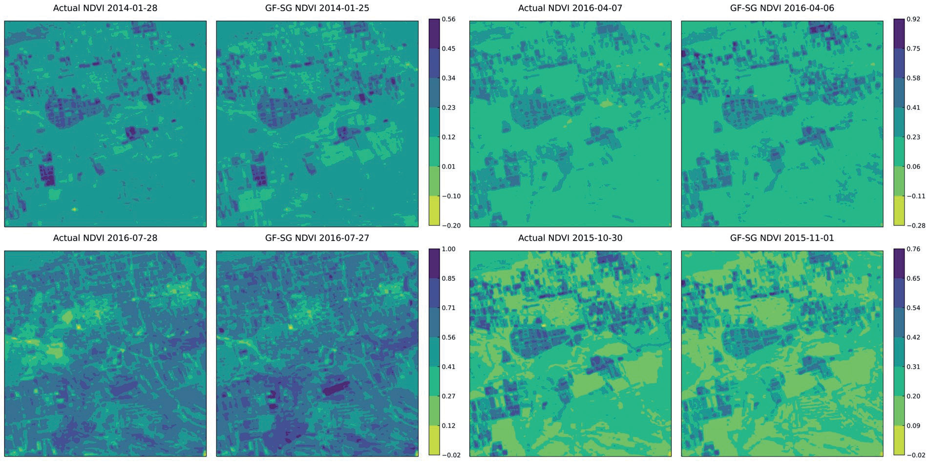
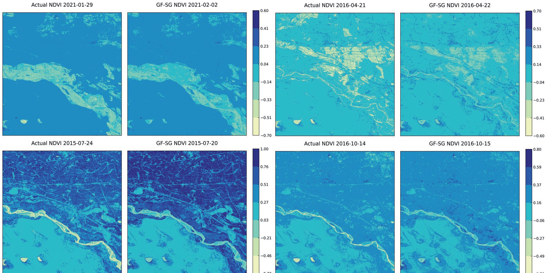
The GF-SG model was adopted for predicting the NDVI time-series data of the research area from 2000 to 2022. The spatial coverage included Landsat images with 12 different paths and rows. To address missing data and cloud contamination, we selected the MODIS-NDVI time series data that matched each path and row. Through the synthesis of GF-SG composite NDVI, it was found that taking the maximum value in overlapping areas provides a smoother transition effect compared to taking the minimum value or the mean. Therefore, for the stitching of 12 scenes of GF-SG NDVI data, the maximum value of NDVI in overlapping areas of different row and column numbers was selected. After masking, we obtained an 8-day 30 m resolution NDVI time series for a specific area from 2000 to 2022. We compared the accuracy of the NDVI images obtained by applying the GF-SG model with that of Landsat NDVI images without cloud cover for similar dates, as shown in Table 1 and Figs. 3 and 4. The accuracy comparison for the selected comparison image path and row numbers were (126, 32) and (128, 32), respectively, in the eastern and western parts of the research area. The selected dates for data within the range of (126, 32) were January 28, 2014, April 7, 2014, July 28, 2016, and October 30, 2015. For the range of (128, 32), the selected dates were January 29, 2021, April 12, 2016, July 24, 2015, and October 14, 2016. These dates corresponded to the four seasons of winter, spring, summer, and fall in the study area. The verification area exhibited a 5.5 km × 5.5 km range, encompassing various land covers such as riverbanks, urban areas, farmland, and grassland. The spatial detail simulation results showed that the NDVI predicted by the GF-SG model preserved the details of grassland, farmland, and urban area boundaries. The overall spatial trend of NDVI was consistent with that of Landsat NDVI without cloud contamination.
Table 1.
GF-SG Simulated NDVI Verification Dates.
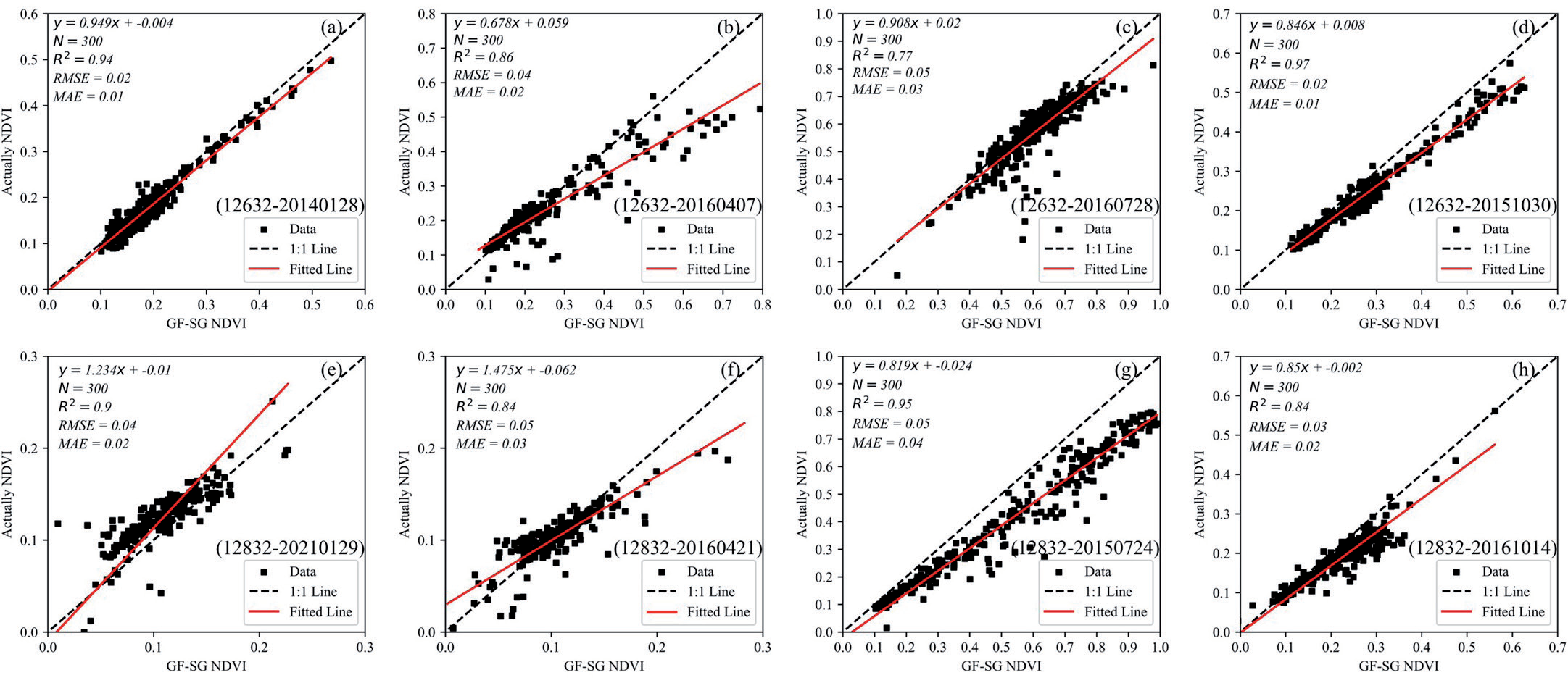
In the selected area, 300 sampling points were randomly generated using ArcGIS 10.7, and the corresponding NDVI data of the grids were extracted for accuracy evaluation (Fig. 5). The x-axis denotes the NDVI values predicted by the GF-SG model, and the y-axis represents the NDVI values extracted from the actual Landsat data. The dashed black line denotes the 1:1 line. Most of the data points were scattered on both sides of the line. The R2 values range from 0.77 to 0.97, RMSE ranges from 0.02 to 0.05, and MAE ranges from 0.01 to 0.04, all close to 0. The GF-SG model predicts NDVI values for various seasons, showing slightly poorer predictions in April but results closer to the true cloud-free Landsat NDVI data in October, with excellent simulation accuracy across different land covers in the research area.
Fig. 3.
Comparison between the merged NDVI image and the original NDVI image for the region with path-row number (126, 32).
Simulation Results of the PT-JPL Model
The sensitivity parameters 𝑘1 and 𝛽 of the PT-JPL model were calibrated using eddy covariance estimated ET data from 2015 to 2016. By iterating through the model with set step sizes and upper and lower bounds, the optimal parameters were selected. The input parameters corresponding to other land types refer to the conclusions of Shao et al. [26]. The model was validated using eddy covariance data from 2016 to 2017. Table 2 presents the optimized parameters of the PT-JPL model for grassland and shrubland land use types. Fig. 6 illustrates the accuracy evaluation of the model from 2015 to 2017, with the y-axis representing the actual observed ET values at the eddy flux sites and the x-axis representing the estimated values of ET. The red lines represent the fitted trend lines, and the dashed black lines denote the 1:1 line. During the calibration period, the simulated ET accuracy of PT-JPL ranged between 𝑅2 values of 0.88-0.91, RMSE values of 0.57- 0.60 mm/day, and MAE values of 0.38-0.46 mm/day. In the validation period, the simulated ET accuracy ranged between 𝑅² values of 0.85-0.87, RMSE values of 0.54- 0.72 mm/day, and MAE values of 0.36-0.47 mm/day. The study area, located in a semi-arid region, primarily exhibited ET values ranging between 0-1 mm/day. The model performed more accurately for low ET values but presented greater dispersion and relatively higher errors for values between 2–4 mm/day. However, overall, the simulated values were consistent with the observed trends. Fig. 7 illustrates the ET comparison for each 8-day period from 2015 to 2017. Before optimization, the PT-JPL model tended to provide higher estimated ET results for grasslands and shrublands, especially in March and April of each year. Following optimization, the ET simulation of the PT-JPL model aligned more closely with the actual observations over the time series, reducing the overestimation of ET values.
Table 2.
Optimization of the parameters for the PT-JPL model across different underlying surfaces.
| Land classification | k1 | β |
|---|---|---|
| Grassland | 0.64 | 1.02 |
| Shrubland | 0.71 | 1.29 |
Temporal and Spatial Variations of Evapotranspiration in the Yellow River Basin of Inner Mongolia
The interannual variation in ET is shown in Fig. 8. The annual ET changes exhibited a fluctuating increase in the multi-year average evapotranspiration, ranging from 226.26 to 373.84 mm with a span of 147.58 mm. The maximum ET occurred in 2003, while the minimum occurred in 2005, with a multi-year average ET of 304.18 mm. Analyzing ET on an 8-day basis, the maximum daily evapotranspiration for the prior 23 years was 3.42 mm, with a minimum of 0.0014 mm.
Fig. 9 shows the spatial distribution of the multiyear average ET and its components. The multi-year average ET ranged from 17.18 to 633.96 mm, showing a decreasing pattern from west to east. High ET areas were concentrated in irrigation areas, farmland, and mountainous forest areas in the eastern part of the basin, whereas low ET areas were concentrated in the western part, including the Ulan Buh and Kubuqi Deserts. The spatial trend of Ec was aligned with the high-value areas of ET, with low-value areas mainly in the desert and western mountainous areas of the basin. The Ei had relatively small values throughout the study area, with high values appearing in the eastern mountainous forest areas. Es was low in agricultural irrigation areas, western mountainous areas, and desert areas, whereas high values occurred in natural grasslands in the basin.
Fig. 10 illustrates the spatial trends in the annual ET and its components. The proportion of areas exhibiting increasing trends in ET was 49.1%, whereas those with decreasing trends represented 48.7%. Approximately 82% of the basin area showed no significant change in ET. There were notable differences in the trend of ET among different land use types, with 79% of unused land demonstrating a significant decrease and 56% of shrubland presenting a significant increase, while grassland, cropland, and forest land showed no significant trend change.
Regarding the annual Ec in the research area, regions with increasing trends accounted for 75.9%, with 54.65% being significant. The significance level of the trend in Ec increased from west to east. The regions with significant decreases in Ec were primarily distributed near lakes and rivers, and on the outskirts of cities. The annual Ei in the eastern part presented a significant increasing trend, whereas the Ei in the middle and western parts of the basin exhibited a significant decreasing trend. The spatial trend changes in the annual Es were aligned with those of ET.
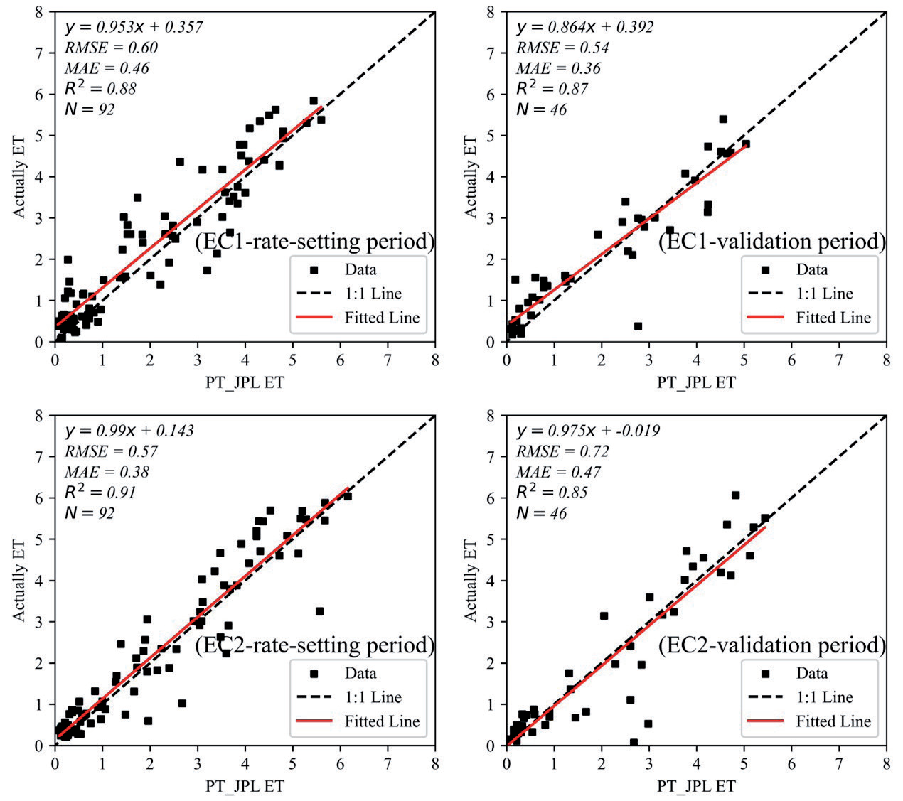
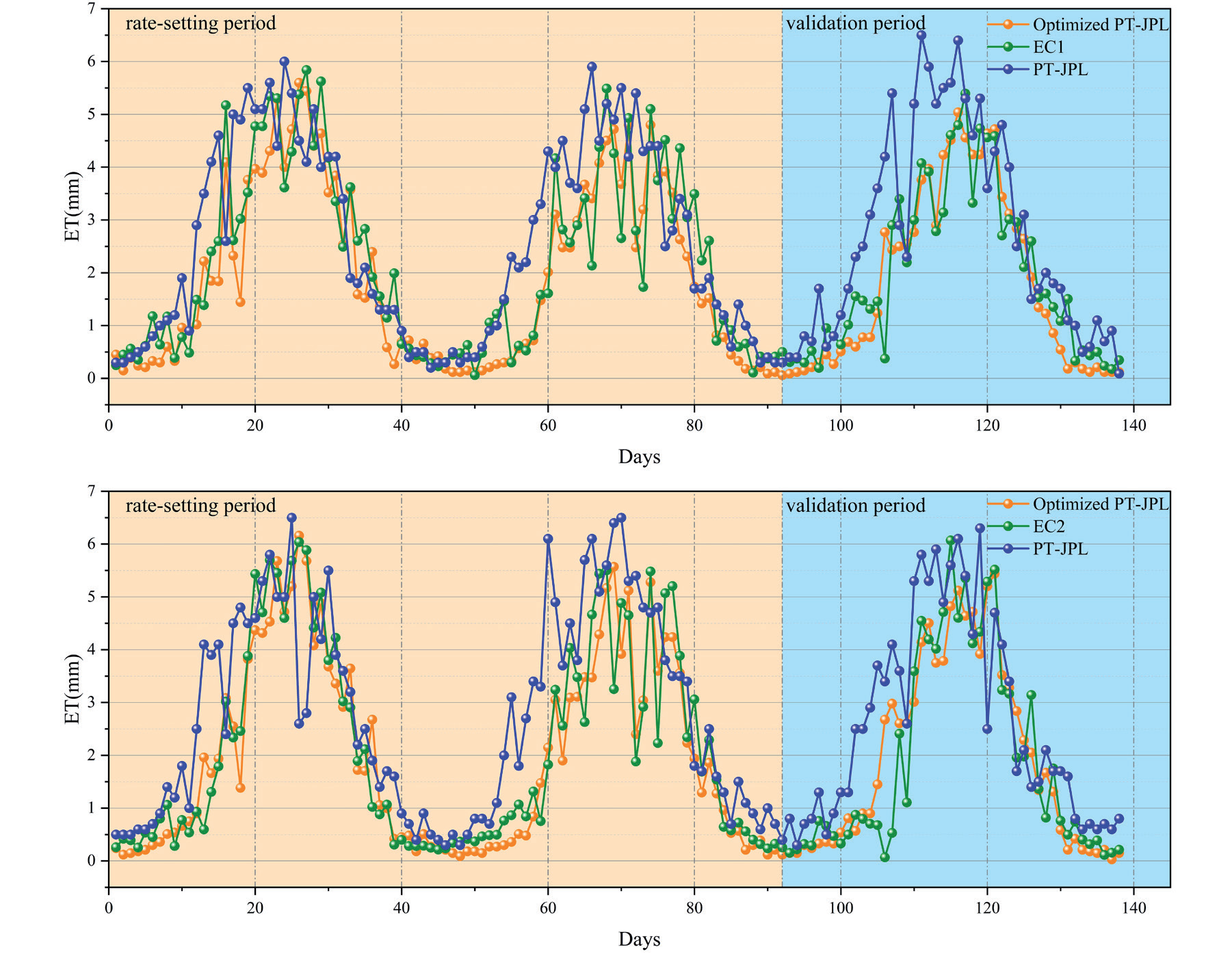
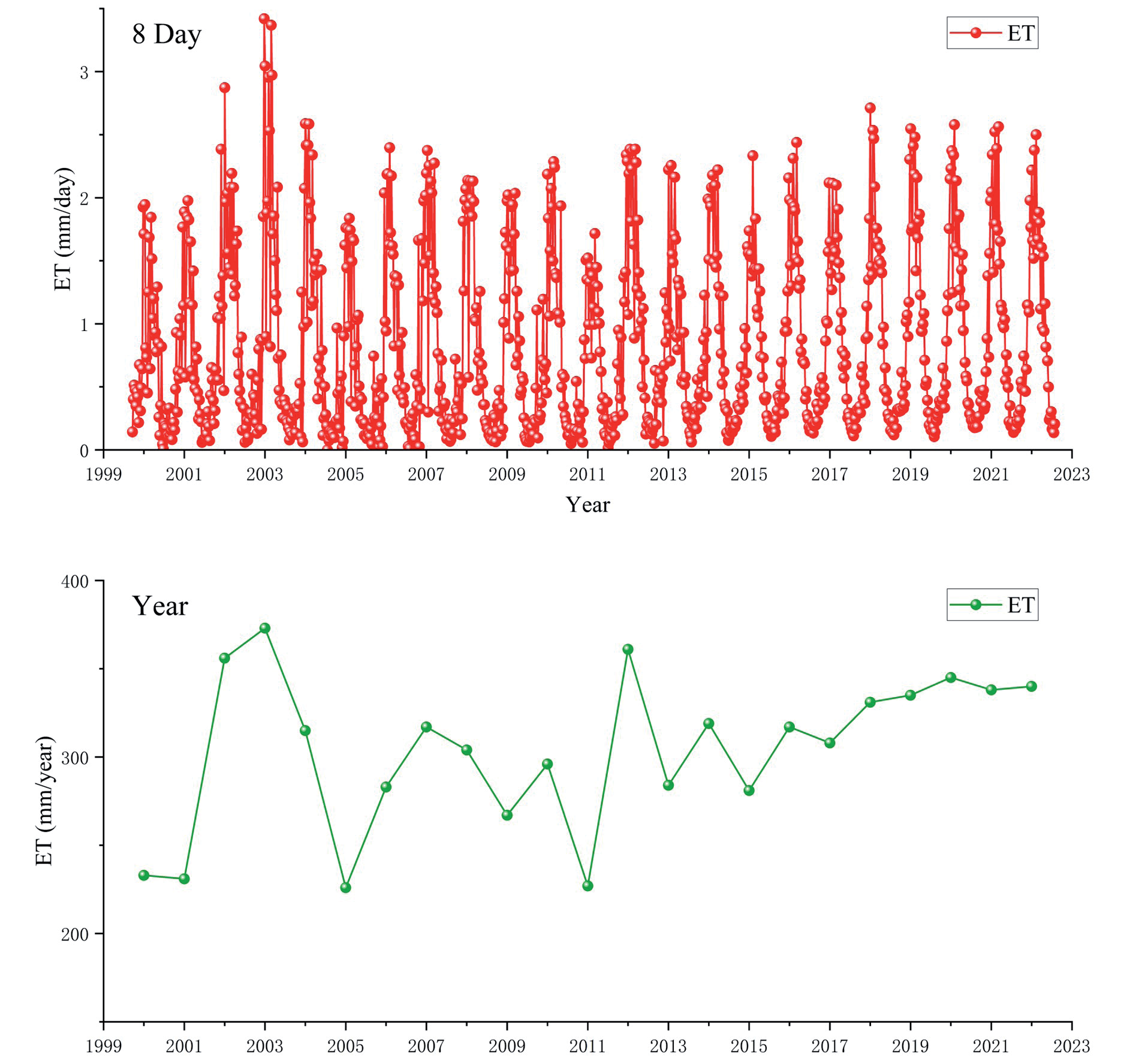
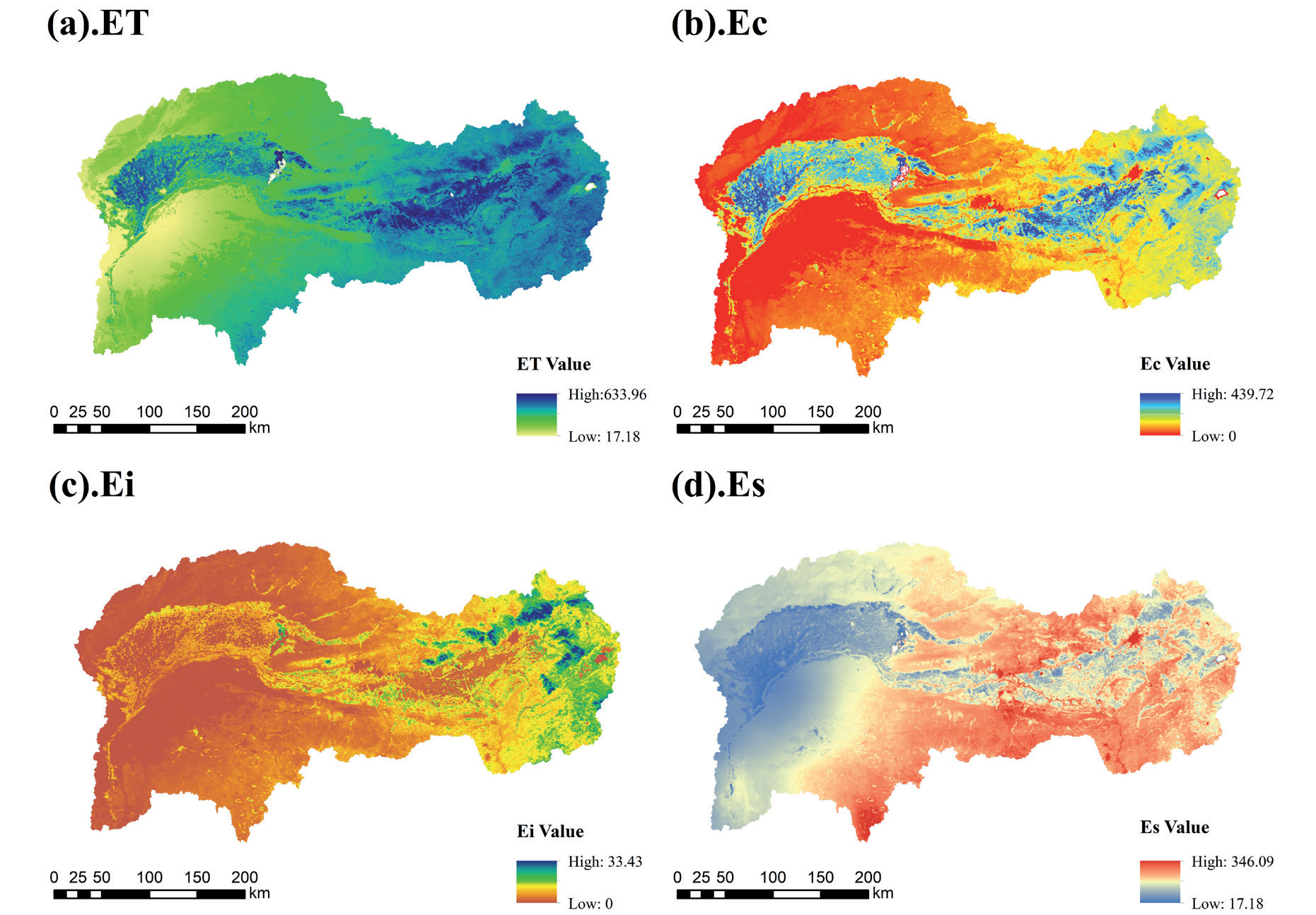
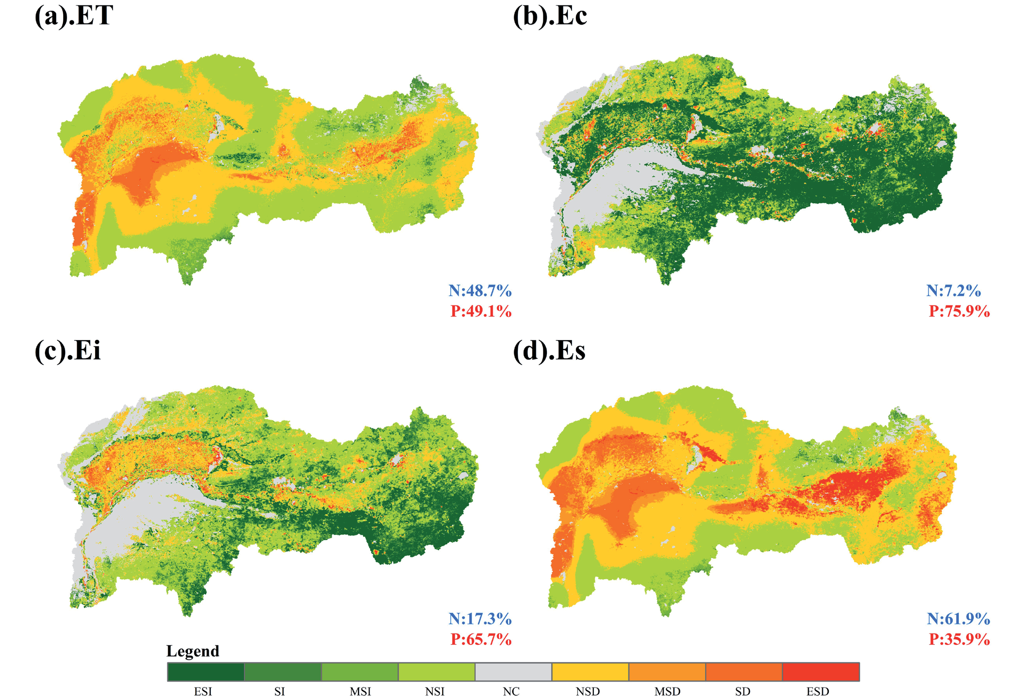
Table 3.
Statistical analysis of changes in evapotranspiration trends.
Spatial Continuity of Evapotranspiration (ET) Variations in the Study Area.
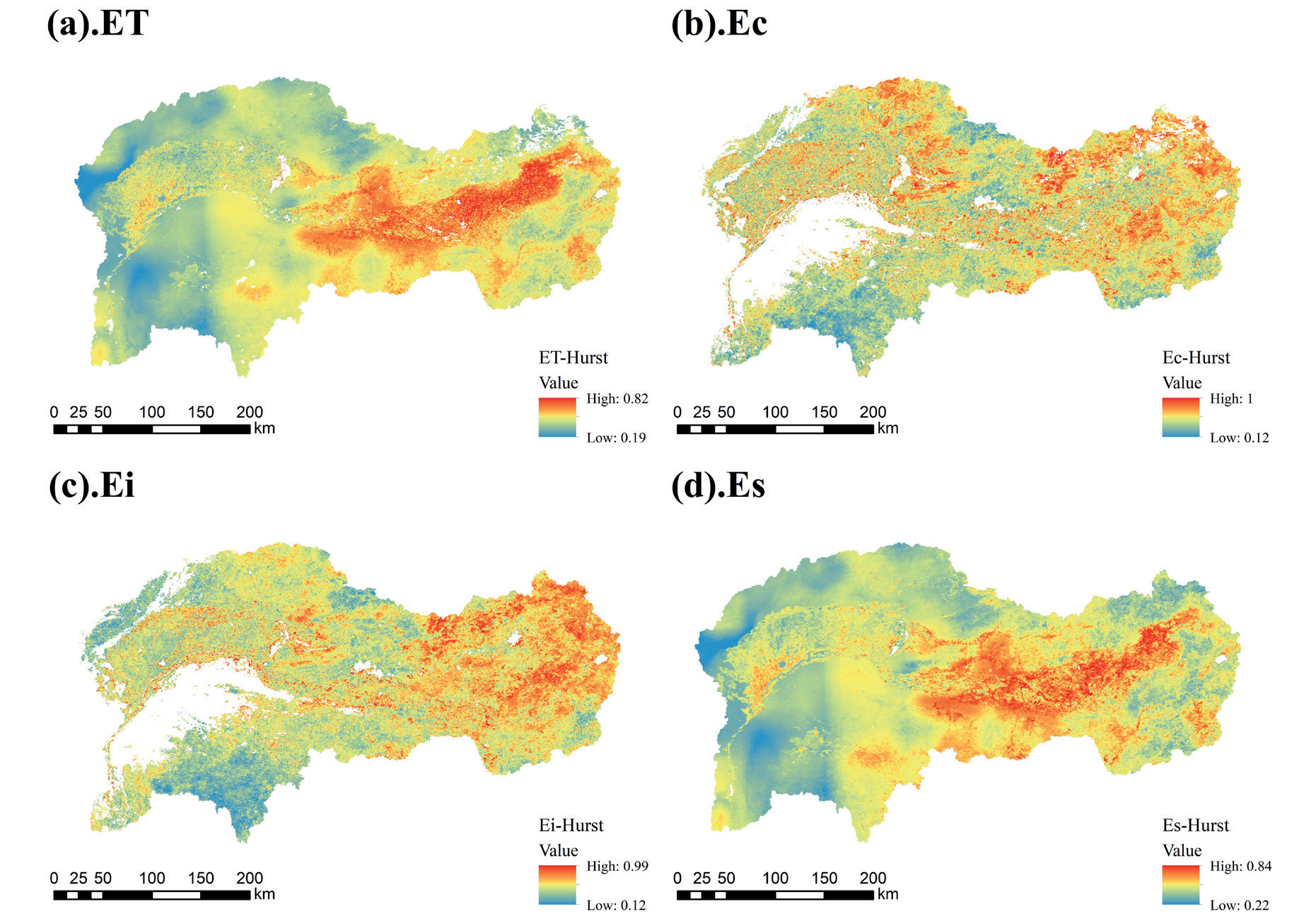
The spatial pattern of the Hurst index of annual ET in the specified area exhibited high and low values in the east and west, respectively (Fig. 11), with a mean value of 0.44. Approximately 77.61% of the Hurst index values ranged from 0 to 0.5, indicating anti-persistence. They were mainly concentrated in the western part. The Kunlun River Basin, Shidaikongdui River Basin, and Dahei River Basin in the eastern region exhibited pronounced persistent trends in ET. The spatial distribution of the Hurst index for Es closely resembled that for ET. The Hurst index for Ec and Ei presented a generally consistent spatial distribution, with values in the range of 0.5–1.0 concentrated in the eastern part, particularly in the Dahei and Hun River basins. The areas with Hurst values in the range of 0-0.5 were predominantly located in the southwestern part of the basin, namely the Xue’erduosi Plateau region.
Table 4.
Analysis of future trends in evapotranspiration.
Combining Sen’s trend analysis with the Hurst index provided insights into the future trends of ET and its components (Table 4). Future trends for ET and Es mostly exhibited anti-persistent changes, with the largest proportion (40.13%) demonstrating an increasing anti-persistent trend, primarily distributed in the southern and northern parts, indicating a continuous decrease in ET over the next 23 years in these regions. In the western part, future ET exhibited a decreasing-anti-persistent trend, accounting for 37.48% of the area, where the trend changed from a decrease to an increase. Overall, 46.44% of the study area demonstrated an increasing trend in ET, whereas 53.56% exhibited a decreasing trend. Ec and Ei presented opposite future trends, with increasing Ec and decreasing Ei.
Impact of Land Use Transitions on Evapotranspiration
Land use dynamics can be a key factor influencing spatiotemporal variations in evapotranspiration and is a principal input parameter for the PT-JPL model. As shown in Fig. 12, in 2022, the area of the study region was 105,000 km2 , with cropland covering 26,400 km2, forestland covering 1,900 km2, shrubland covering 0.007 km2, grassland covering 60,300 km2, water bodies covering 0.085 km2, unused land covering 11,800 km2, and urban land covering 3,000 km2. These land types accounted for 25.26%, 1.82%, 0.0066%, 57.70%, 0.81%, 0.000006%, 11.29%, and 2.87% of the land area in the study region, respectively. Cropland, grassland, and unused land constituted the highest proportions, occupying a dominant position among the land use/cover types, with a combined area accounting for 94.25% of the entire basin.
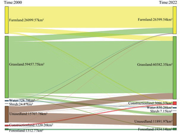
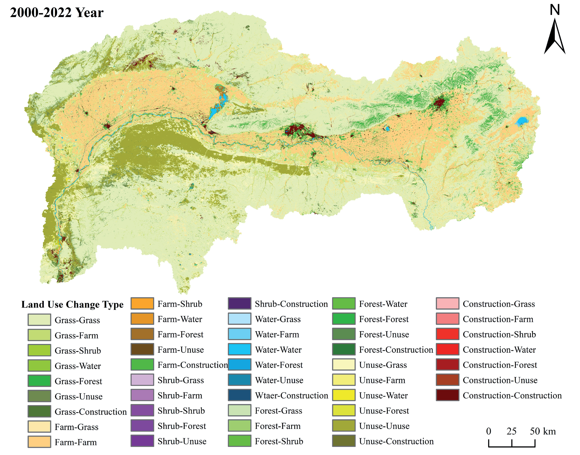
The land-use transfer matrix from 2000 to 2022 is presented in Table 5. The largest increase in land area within the study area was attributed to construction land, with an increase of 1866.12 km2. Most of this increase in construction land area was converted from grassland to farmland, with a growth rate of 152.9%. Grassland has consistently been the land use type with the highest proportion within the basin, with an increase in area of 924.6 km2 over the past 23 years. The largest land type flowing into grassland was unused land, with an area of 3275.12 km2. The area of forest land increased by 47.33%, but a relatively small proportion of land use remained within the basin. The area of unused land within the study area decreased by 24.29%, with most of the unused land flowing into grasslands. However, there is still a significant amount of unused land that has not been effectively utilized.
Fig. 13 illustrates the spatial transfer of land-use changes in the study region. Substantial increases in grassland were primarily observed in the southwestern part, including the West Zhuozi Mountain, West Ordos Plateau, and the Ten Major Loess Gullies, with the largest increase in grassland area located on the south side of the mainstream of the Yellow River. The areas where forest land increased were mostly distributed in the eastern and central parts, including the Daheihe and Hunhe River basins. The outflow of unused land was concentrated in the western mountainous and desert areas. The ecological conditions in areas with low vegetation coverage in the study area have gradually improved.
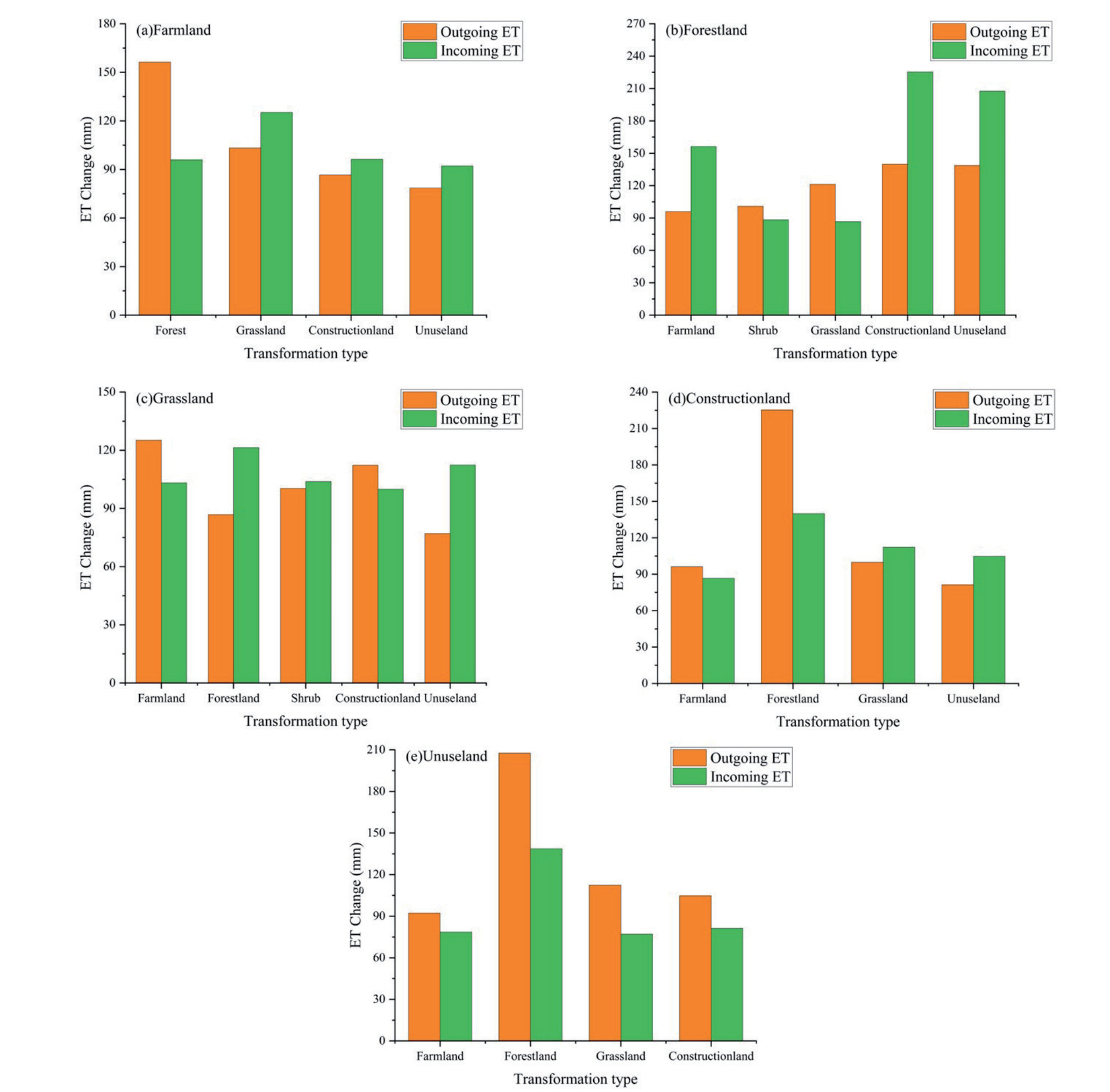
This study compared multi-year ET changes corresponding to different land cover transition areas to elucidate the impact of these transitions on ET. The ET change was calculated by subtracting the ET in 2022 from that in 2000. The land use transition areas with conversion areas exceeding 100 km2 were selected for analysis, considering the variety of land use transition types involved. The selected types were categorized and statistically analyzed against the corresponding ET changes using ArcGIS.
As shown in Fig. 14, from 2000 to 2022, the main land types involved in land use transitions were cropland, grassland, woodland, unused land, and built-up land. The increase in ET from cropland to woodland was 156.34 mm, exceeding the 95.98 mm increase from woodland to cropland. Additionally, ET increases from grassland, unused land, and built-up land to cropland were greater than the corresponding increases from cropland. The increases in ET from unused land, built-up land, and cropland to woodlands exceeded the ET outflows from woodlands. Similarly, the increases in ET from woodland to shrubland and grassland were greater than those after conversion. The increases in ET from grassland to cropland and built-up land were also greater than those after conversion. Moreover, the increases in ET from built-up land to woodland and cropland were greater than the corresponding increases after conversion, with the highest increase observed from built-up land to woodland at 225.37 mm. The transitions from unused land to built-up land, grassland, woodland, and cropland resulted in ET outflow greater than inflow, with the largest increase observed when transitioning from unused land to woodland, at 207.60 mm.
Table 5.
Land Use Transfer Matrix in the study region from 2000 to 2022.
Discussion
Integration of Multi-source Remote Sensing for Evapotranspiration Simulation
The GF-SG spatiotemporal fusion model was used to synthesize high spatiotemporal resolution NDVI time-series data at 8-day intervals and 30 m resolution for the Inner Mongolia Yellow River Basin. The comparisons with the NDVI calculated from cloud-free Landsat images from the same or similar periods presented excellent simulation accuracy. Cao et al. [18] also successfully reconstructed the NDVI time series data for the Qinghai-Tibet Plateau by adopting the GF-SG model, demonstrating its effectiveness for heterogeneous underlying surfaces in arid and semiarid regions. The PT-JPL model was then applied to input vegetation data at 8-day intervals and 30 m spatial resolution. The parameter optimization for the PT-JPL model across different land-use types was performed using data from two eddy covariance stations within the basin. This optimization enabled the simulation of basin-scale ET and its components from 2000 to 2022. The optimized PT-JPL model demonstrated high accuracy for estimating ET in the study area. Shao et al. [26] simulated the ET in the Loess Plateau by applying the PT-JPL, yielding results consistent with those of this study. In the ET simulation results for the Inner Mongolia Yellow River Basin using the PT-JPL model, deviations ranged from to 2–4 mm/day. These deviations were primarily attributed to the concentration of ET in the 3–4 months period, coinciding with the snowmelt season. During this period, NDVI data simulated using the GF-SG model tended to be overestimated, as shown in Fig. 5b and 5f, resulting in a higher ET simulation using the PT-JPL model [20].
Spatiotemporal Variations of Evapotranspiration
The ET regions were concentrated in the Hetao Irrigation Area, farmland areas in Hohhot and Baotou cities, and mountainous forested areas in the eastern part of the basin (Fig. 9). As the largest irrigation area in the Yellow River Basin of Inner Mongolia, The Hetao Irrigation Area diverts water annually from the Yellow River for irrigation, effectively increasing the ET. Often even greater than precipitation. The significant precipitation in the eastern part of the basin promotes lush vegetation growth during the growing season, contributing to the high ET regions. Although there was no significant increase in cultivated land area, ET over cultivated land within the study area increased (Fig. 10), indicating that artificial irrigation was the main factor driving this trend [27]. Low ET regions were primarily identified in the western mountainous and desert areas of the region, where vegetation was sparse, and the primary source of evaporation was Es, owing to scarce precipitation.
The annual ET in the basin exhibited an increasing trend of 2.587 mm/year. Future changes in basin ET (Fig. 11) revealed that areas with persistent ET changes were located in the central and eastern parts, particularly in croplands, shrublands, and forests of Hohhot, Baotou, and Dalad Banner. This suggested that the areas with moderate-to-high-intensity precipitation and robust vegetation growth experienced persistent changes in ET. Table 4 indicates that the most dominant type of future persistent ET change in the basin was the increasing anti-persistent type, primarily found in the western regions, including the West Ordos Plateau and Langshan Mountain area. Recent greening of vegetation in the area has led to an increase in ET, with these artificial covers consuming significant soil moisture. Ongoing vegetation eco-restoration efforts in the western regions of the basin have indicated an original rise and a subsequent decrease in ET trends. This pattern suggested that the extensive development of vegetation restoration projects significantly affected the distribution of water resources [28, 29]. However, the degree of vegetation growth was constrained by soil moisture [30]. Therefore, to maintain the sustainability of socio-economic and ecological development, future ecological restoration projects should consider the threshold of vegetation coverage [31] and carefully strategize the types and densities of vegetation.
Ec represents the key component of ET in the study area and presented excellent consistency with ET in terms of spatial distribution and trend changes. Recent ecological restoration projects have led to a multiyear average Ec distribution of low values in the west and high values in the east, with a significant upward trend. However, the Ec exhibited a notable downward trend near river channels (Fig. 10b). Between 2001 and 2010, land change contributed to a 78.4% decrease in runoff, marking a 10.2% increase compared with 1980–2000 [32]. The “grain for green” program has led to newly planted vegetation requiring more water than natural vegetation [33]. The changes in vegetation patterns can directly alter the distribution of precipitation between runoff and Ec, thereby affecting the distribution of water resources [34]. Extensive vegetation restoration around river channels has disrupted the water resource balance, causing some river channels to dry up, while increased vegetation coverage has sharply raised the Ec, reducing water efficiency and affecting plant survival rates, ultimately decreasing the Ec around river channels. Studies have indicated that the land-use change relative to the water balance is increasing [35], with forests serving as the primary source of canopy interception. Over the past 23 years, the increase in forest area has significantly increased annual Ei in the eastern region. Conversely, the Ei in the river irrigation areas of the central and western basins notably decreased. The Hetao Irrigation Area relies heavily on the Yellow River water because of its low precipitation. However, the long intervals between irrigations with Yellow River water often fail to meet crop growth needs [36]. Historically, flood irrigation has been common in the Hetao Irrigation Area and has led to significant water waste [37]. Recently, this area has promoted the “Yellow River Drip Irrigation” Project [38], which diverts water from the Yellow River to sedimentation reservoirs through existing channels and lakes. The water is then lifted and pressurized by pumping stations and transmitted through pipelines to the fields for irrigation. This project integrates water and fertilizer management, reduces Ei, and significantly improves water-use efficiency in the Hetao Irrigation Area.
Impact of Land Use Change on Evapotranspiration
Over the previous three decades, the Chinese government has launched numerous large-scale vegetation restoration projects such as the Three-North Shelter Forest Program, alongside various local initiatives [39]. These efforts have been prompted by the extensive LUCC in China, which has resulted in environmental ecological issues, including soil aridity and reduced runoff [40]. This study calculated the land use type transition matrix for the years 2000-2022 based on CLCD land use data (Table 5), and the resulting changes in ET induced by land cover type transitions were determined (Fig. 13). Land use conversion from 2000 to 2022 positively affected ET in the study area. Over the past 23 years, significant mutual conversions have occurred among grassland, woodland, cropland, and unused land, with increases observed in most land types, except for unused land and shrubland. The majority of land type conversions have occurred in the western region, such as the Western Zuozi Mountain, Western Ordos Plateau, Wolf Mountain, and Ser Ten Mountain, where ET conversion rates are higher than those in other areas. Among the various land-use type changes, woodland conversion had the greatest impact on ET changes. Woodlands typically possess a deeper root distribution, larger leaf area, and deeper root distribution, making deforestation and afforestation the most influential LUCC processes affecting ET changes [41]. When woodland is converted to farmland or grassland, there is also a higher ET increment, possibly because of the presence of many stunted trees with poor growth due to water shortages in the basin. The conversion of these areas to grassland or farmland results in a faster growth cycle, leading to increased ET. The order of water consumption derived from the study was woodland > cropland > construction land > grassland > unused land, providing a reference for future regional ecosystem planning.
Conclusions
This study performed high-precision retrieval of ET in the Inner Mongolia Yellow River Basin between 2000 and 2022 at 8-day intervals and 30-meter spatial resolution using GF-SG combined with the PT-JPL model. The spatiotemporal characteristics of ET and its components were analyzed, with the influence of land use changes on ET for the period 2000-2022 explored. The main conclusions are as follows.
(1) The GF-SG time series interpolation model showed high accuracy in predicting NDVI, particularly in delineating the boundaries of grassland, cropland, urban areas, and water bodies. It accurately estimated the NDVI time series over large regions with complex underlying surfaces, thereby saving time and computational resources.
(2) Integrating high spatial and temporal resolution vegetation data with spatially interpolated meteorological data into the PT-JPL model and optimizing three sensitive parameters (k1, β, and Topt) resulted in improved simulation accuracy. The analysis of spatiotemporal variations in ET in the study area revealed a west-to-east decreasing trend in the overall spatial distribution, with high-value areas primarily in the Dahei, Hun, and Kundulun River basins. Regions with high values of Ec were distributed in the Hetao Irrigation Area, whereas areas with high values of Ei were identified in forested regions, predominantly in the Dahei and Hun River basins. The spatial distribution pattern of the Hurst Index for ET showed a west-to-east decreasing trend. The future trend of ET mainly exhibited an increasing antipersistent pattern.
(3) Cropland, grassland, and unused land were the dominant land use categories in the study region. Grasslands had the largest area and showed the most significant growth trend, primarily from conversions from cropland and unused land. Although forestland saw the greatest proportional increase, it still represented a relatively small part of the basin's total area. Construction land was mainly converted from grassland and cropland, whereas forestland was primarily found in the Dahei River basin in the eastern region, and cropland was concentrated along the main river. The patterns of ET increments in different land use/cover transfer areas were as follows: ET increment in forestland > ET increment in cropland > ET increment in construction land > ET increment in grassland > ET increment in unused land.