

Introduction
With the intensification of global climate change and human activities, the ecological environment is facing unprecedented challenges. The health status of ecosystems is directly related to the maintenance of biodiversity, sustainable utilization of resources, and the guarantee of human well-being. Therefore, effective monitoring of the ecological environment, timely detection, and response to abnormal changes have become a key task for global environmental protection and sustainable development. Natural resources provide the necessary material basis for human survival, so the sustainable use of natural resources is the premise of ensuring the sustainable development of human society. The change of natural resources is determined by the structure and functional state of the ecosystem, the operation status of the ecosystem process, and the effectiveness of ecosystem management. The purpose of studying ecosystems and ecological processes is to make more rational use of natural resources. Regarding the issue of resource utilization, some scholars have established an evolutionary game model between industrial enterprises, local governments, and central governments, analyzing the dynamic interaction between vertical decentralization, environmental regulation, and corporate pollution. This provides valuable insights for developing countries seeking to improve their governance capabilities throughout the entire green transformation process [1]. Not only that, green technology innovation is a key force in promoting green development, and relevant scholars have used the difference in differences model to evaluate the impact of ecological civilization construction on green technology innovation. Research has found that the construction of ecological civilization has significantly promoted the innovation of green technology in the experimental zone. Due to the positive spatial spillover effect of green utility model patents and the negative spatial spillover siphon effect of green invention patents, the promotion effect on green utility model patents is greater. The construction of ecological civilization not only has direct effects, but also brings about environmental investment and human capital. In addition, it also helps to strengthen industrial infrastructure and organizational structure, thereby improving the innovation level of green technology. Ecological environment symbiosis monitoring is the foundation of ecological environment protection and an important support for ecological civilization construction. For accurate monitoring, the data quality must be ensured. The collection, processing and analysis of monitoring data directly affect the results of ecological environment symbiosis monitoring. For this reason, several long-term ecosystem research networks have been established in the world. These networks have carried out various experiments, observations, and studies based on network-based long-term positioning observation, and accumulated a large amount of data in various formats. There are abnormal elements in these data, which directly affects the accuracy of ecological environment symbiosis monitoring [2, 3]. Symbiotic monitoring data not only covers the interactions between organisms and the environment but also the interdependence between biological populations, providing valuable information for understanding the stability and resilience of ecosystems. However, due to the complexity and variability of ecosystems, monitoring data often contains various abnormal signals, which may be manifestations of natural fluctuations or early warnings of ecosystem degradation or destruction. Therefore, conducting research on abnormal monitoring and modeling of ecological environment symbiosis monitoring data has important scientific significance and practical value for improving the accuracy and reliability of monitoring data and timely identifying potential risks of the ecosystem. Intended to establish effective anomaly monitoring models, reveal anomaly patterns in symbiotic monitoring data, and provide scientific basis and technical support for the protection and management of ecosystems. This study is expected to provide decision-makers and technicians in the field of ecological environment monitoring with a practical set of tools to cope with increasingly severe ecological environment challenges and promote harmonious coexistence between humans and nature. Therefore, studying abnormal monitoring methods for ecological environment symbiosis monitoring data is of great significance.
In the research [4], the sensitivity of co-dispersion to noise and error in ecological environment data is studied, and Monte Carlo simulation and real data sets are used to study the sensitivity of co-dispersion to four common pollutants in many forest data sets. A useful method for filling in missing spatial data is also proposed. In the research [5], a new energy field abnormal data mining method based on an improved Adaboost algorithm is proposed. After preprocessing the new energy field data, the algorithm is improved by introducing dynamic weight parameters to solve the shortage of the Adaboost algorithm. After calculating the abnormal degree of the data with the direct inference confidence machine, the neural network is used to reduce the error value of the Adaboost algorithm. Finally, the output of the Adaboost algorithm is used to realize abnormal data mining. In the research [6], abnormal data are divided into three types: numerical anomaly, fluctuation anomaly, and abnormal event. Based on the anomaly detection algorithm of regression residual probability distribution, a data preprocessing method for coastal wetland ecological observation is constructed by using look-up tables and multi-index time series model and integrating the relationship between multiple environmental factors. Ji et al. [7] established the MSLSTM (multi-scales long short-term memory) model to predict the index data, and then established the DA (dual-stage attention-based) model based on the residual distribution of the prediction results, and determined the data anomaly threshold of each index. When the difference between the measured data and the predicted data is greater than the threshold value, it is determined as abnormal data. This method cannot accurately monitor temperature data and humidity data and has the problem of low monitoring accuracy. Ji et al. [8] used the RDU (region dual-channel unit-linking) algorithm to downsample the majority of class data and remove duplicate samples, and used the SMOTE (synthetic minority over-sampling technique) algorithm to oversample the minority of abnormal data. The imbalance of the data set is improved by the synthesis of new abnormal data, and then the abnormal data monitoring model is obtained by training the RF (random forest) classification algorithm. This method requires a long time of data monitoring and has the problem of low monitoring efficiency. Zhang et al. [9] extracted the trend term of monitoring data through wavelet transform, and then used the isolation forest algorithm to identify the outliers of the remaining amount after deducting the trend term. This method has a low rate of detection and a high rate of false detection.
Ecological environment symbiosis monitoring data may be affected by various factors, such as instrument errors, improper operation, data processing errors, etc., which can lead to low data quality and thus affect the accuracy of anomaly monitoring. Moreover, the amount of data involved in ecological environment monitoring is usually very large, including monitoring data of various environmental factors (such as atmosphere, water, soil, biology, etc.), which have complex interactions and impacts, increasing the difficulty of anomaly monitoring. Due to the existence of these difficult problems, the above methods have problems such as large differences between monitoring results and reality, long average operation time, low detection rate, and high false detection rate in the application process. Therefore, through density clustering, large-scale and complex datasets can be processed, and clusters and outliers in the data can be automatically identified without specifying the number of clusters in advance, thereby improving the quality of detection and monitoring. The existing research on density clustering algorithms mainly focuses on the outlier detection of power load data. Usually, adaptive parameters and cluster centers are automatically selected, and then big data outliers are evaluated through standardized local density and distance to finally find outliers. However, the selection of simple adaptive parameters and cluster centers is not enough to make up for the judgment of dataset parameters when data is missing, which will affect the estimation accuracy. Therefore, in this paper, a genetic algorithm is used to estimate the parameters of incomplete data, and a Markov chain is generated when missing data is supplemented to improve the convergence performance and obtain complete distributed data. This approach can improve the estimation accuracy of incomplete data parameters, and then optimize the monitoring effect of ecological environment symbiosis monitoring abnormal data. However, ecological environment symbiosis monitoring data is usually multidimensional, and density clustering-based methods can effectively process multidimensional data by considering the relationships between multiple variables to identify anomalies. This method can reveal complex patterns and correlations in the data and improve the accuracy of anomaly monitoring.
Since the purpose of this study is to improve the monitoring accuracy and efficiency of abnormal monitoring data, as well as reduce the false detection rate of abnormal monitoring data, the assumptions made in this study are as follows:
(1) The monitoring data of ecological environment symbiosis are cleaned up by combining adaptive moment estimation and random gradient descent algorithm. Assuming that only one data is selected from the data set for accurate calculation during parameter optimization can improve the iteration speed and thus have a positive impact on the monitoring efficiency of abnormal data.
(2) A genetic algorithm is used to estimate the parameters of missing data. It is assumed that expanding the range of parameters to be estimated can improve the convergence performance when solving data parameters, so as to obtain a better solution, which will have a positive impact on the monitoring accuracy of abnormal data.
Experimental Procedures
Preprocessing of the Symbiosis Monitoring Data of Ecological Environment
Data Cleaning
There is a large amount of symbiosis monitoring data in the ecological environment. The existing “dirty data” and missing data will have an impact on the abnormal monitoring results of symbiosis monitoring data in the ecological environment. Therefore, it is necessary to clean the symbiosis monitoring data of the ecological environment. The modeling research method for abnormal monitoring of symbiosis monitoring data in the ecological environment based on density clustering adopts a hybrid algorithm combining random gradient descent and adaptive moment estimation to clean the ecological environment symbiosis monitoring data.
(1) Random gradient descent optimization algorithm
Generally speaking, the data expression ability increases with the increased complexity of the deep neural network. The training complexity of the network increases linearly with the complexity of the network. In order to find the global optimal solution in network training, the network parameters must converge to the optimal value. However, the effect of parameter optimization is often affected by the complex structure of deep neural networks. Therefore, it is necessary to propose a general optimization algorithm that can adapt to various network structures.
Random gradient descent is a network parameter optimization algorithm commonly used in deep learning. When updating parameters, only one data is selected from the data set for accurate calculation each time, which greatly speeds up the iteration speed and achieves good results in multiple parameter adjustment experiments. The stochastic gradient descent algorithm optimizes the parameter ϑ at time t as follows:
Where, β is the learning rate; ht is the initial gradient; p(ϑ) is the objective function, and Δϑt is the descending gradient.
The learning rate used by the stochastic gradient descent algorithm to update the parameters is single and has no adaptability to the parameter category. For example, the updating speed of infrequent parameters is accelerated, and the updating speed of frequently occurring parameters is reduced, resulting in each iteration not being able to be carried out in the direction of parameter optimization and not meeting the training requirements of high-speed and low memory [10–13].
(2) Adaptive moment estimation method
As an algorithm for optimizing random objective functions, adaptive moment estimation automatically obtains the appropriate learning rate for each parameter by estimating the first and second moments of the gradient, without manual control [14–16]. It is conducive to improving the convergence speed, accelerating the calculation efficiency, and reducing the memory demand. It is very suitable for training data sets containing large-scale data or parameters to meet the optimization requirements [17, 18]. The adaptive moment estimation algorithm optimizes the parameter ϑ at time t as follows:
Where, kt is the initial gradient, q΄t and m΄t are weighted averages of the first-order moment estimation and the second-order moment estimation, respectively. qt and mt are weighted biased square deviations of the first-order moment estimation and the second-order moment estimation, respectively. χ1 and χ2 are hyperparameters controlling the first-order moment estimation and the second-order moment estimation, respectively. ϕ is the smooth top; Δϑ΄t is the descending gradient.
The objective function of the adaptive moment estimation algorithm in the high-dimensional space often has high and low fluctuations, resulting in the disappearance of the descending gradient and the inability to achieve fine-tuning. In addition, its parameter adjustment process is relatively simple, and it only selects the default parameters to optimize the problems that occurred in the training process. It cannot update the gradient of too large parameters, affecting the effect of data iteration. A long time is taken by the algorithm to optimize and the training efficiency is low [19, 20].
(3) Construction of a stack noise reduction self-encoder model based on adaptive moment estimation and random gradient descent hybrid optimization
For enabling the deep neural network model to converge quickly and effectively avoid the local optimal solution, according to the advantages and disadvantages of adaptive moment estimation and random gradient descent optimization algorithm, the combination of the two is applied to the stack noise reduction self-encoder model [21, 22] to build a stack noise reduction self-encoder model AS-SDAE with adaptive moment estimation and random gradient descent hybrid optimization. In the early stage of AS-SDAE model training, the adaptive moment estimation algorithm is used to converge to a stable trend quickly, and then it is automatically converted into a random gradient descent algorithm after a certain round of training for precise tuning in the later stage [23–25].
Set the parameter S to be optimized, the objective function l(s), the initial learning rate β, and the total number of iterative training ξ(ξ = ξ1 + ξ2 + … + ξt + … + ξr).
The steps of the AS-SDAE model optimization algorithm are as follows:
(1) The objective function gradient of the parameter s under the adaptive moment algorithm is calculated:
(2) The first-order moment estimate qt and the second-order moment estimate mt of the parameters in the adaptive moment algorithm are calculated:
Where, x=0, χ1 = 0.9, x=1, χ2 = 0.99.
(3) The descent gradient Δs't of the current round is calculated:
(4) The descent gradient Δs't obtained in step (3) is returned to step (2) and substituted into kt to calculate the first-order and the second-order moment estimation again, and the iteration of step (2) and step (3) is repeated to update the descent gradient, and the moving average value μt of the adaptive moment algorithm after each iteration is calculated:
(5) When the difference between the biased square difference of the moving average and the initial learning rate after the iteration is updated to round ξt is less than the step ϕ(ϕ = 10-8), the updating of the descending gradient and the moving average is stopped:
At this time, the adaptive moment algorithm has optimized the parameters to a stable trend and switched to the random gradient descent algorithm for further optimization.
(6) In the later ξt+1 to ξr rounds, the moving average value of the adaptive moment algorithm is used as the estimation value of the learning rate of the random gradient descent algorithm, and the descent gradient Δs't after the optimization of the random gradient descent algorithm is calculated:
(7) When the descent gradient after the iteration is updated to a certain round reaches a constant value, completing the optimization of the random gradient descent algorithm, that is, the overall optimization of the parameters of the model is completed.
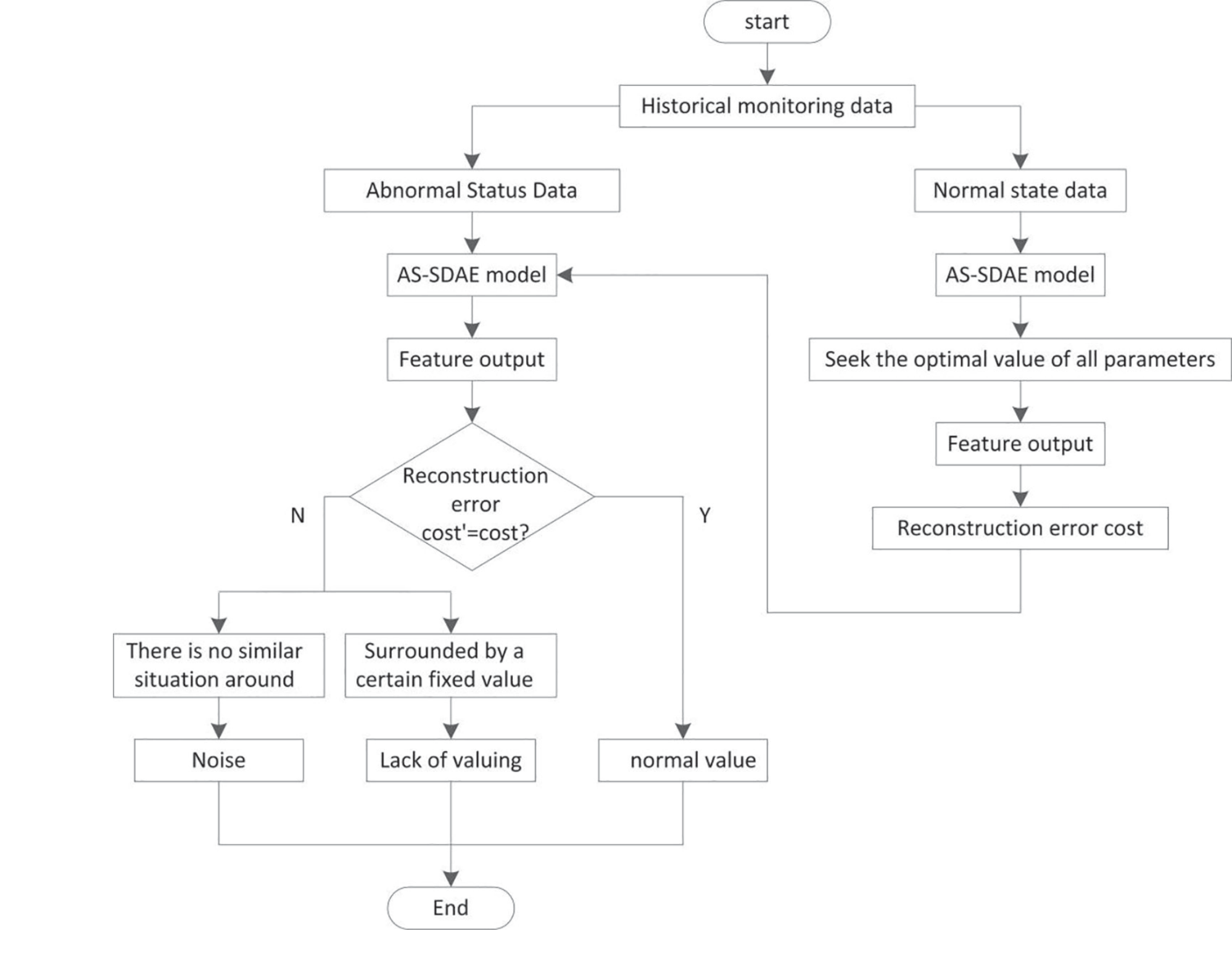
To sum up, the process of cleaning “dirty data” based on AS-SDAE for symbiosis monitoring data of the ecological environment is shown in Fig. 1.
Through the above process, the “dirty data” and missing data in the symbiosis monitoring data of the ecological environment are cleaned out, and the dirty data are deleted directly. The missing data is filled by the following contents.
Missing Data Filling
The data for ecological environment symbiosis monitoring often comes from multiple different sources and formats, and these data sources may have missing values in the data due to various reasons. The presence of missing values can disrupt the integrity of data and affect the reliability of subsequent analysis. Therefore, after cleaning and processing the ecological environment symbiosis monitoring data in previous section, missing data is filled in to ensure data quality to the greatest extent possible. This helps to more accurately reveal the characteristics and patterns of the ecological environment, and improve the accuracy and credibility of the analysis results. The research method for abnormal monitoring modeling of symbiosis monitoring data in the ecological environment based on density clustering uses the Markov chain Monte Carlo method [26, 27] to supplement the missing data of symbiosis monitoring data in the ecological environment. This method is based on incomplete data sets and parameters of incomplete data, and performs iterative estimation on missing data. Because the parameters of the data set cannot be determined due to the missing data, the parameters of the entire incomplete data need to be estimated before filling the missing data. Moreover, the closer the estimated parameters are to the actual values, the closer the estimated missing data are to the real values [28, 29]. In order to improve the effectiveness of the parameters, the proposed method uses a genetic algorithm to estimate the parameters. The main reason is that when dealing with missing data, due to the incompleteness of the dataset, it is not possible to directly determine the key parameters that affect the data-filling effect. In order to improve the accuracy and reliability of filling data, it is necessary to estimate these parameters. A genetic algorithm has become an ideal choice for estimating these parameters due to its global search ability, strong adaptability, parallelism, robustness, and adaptability. A genetic algorithm can perform global search in complex parameter space, find the optimal or approximately optimal parameter configuration, and it does not require high specific form requirements for the problem, and can adapt to various types of problems. In addition, the parallelism and adaptability of genetic algorithms help improve search efficiency and cope with noisy data. Therefore, using genetic algorithms for parameter estimation can effectively improve the quality of missing data filling.
(1) Estimated data mean and covariance matrix
In the symbiosis monitoring data of the ecological environment, the data distribution is mainly divided into two categories: normal distribution and power-law distribution. When estimating the parameters of incomplete data, the proposed method uses the log-likelihood function of the data as the objective function to establish the estimation model, where the mean and variance matrix are the parameters [30–32].
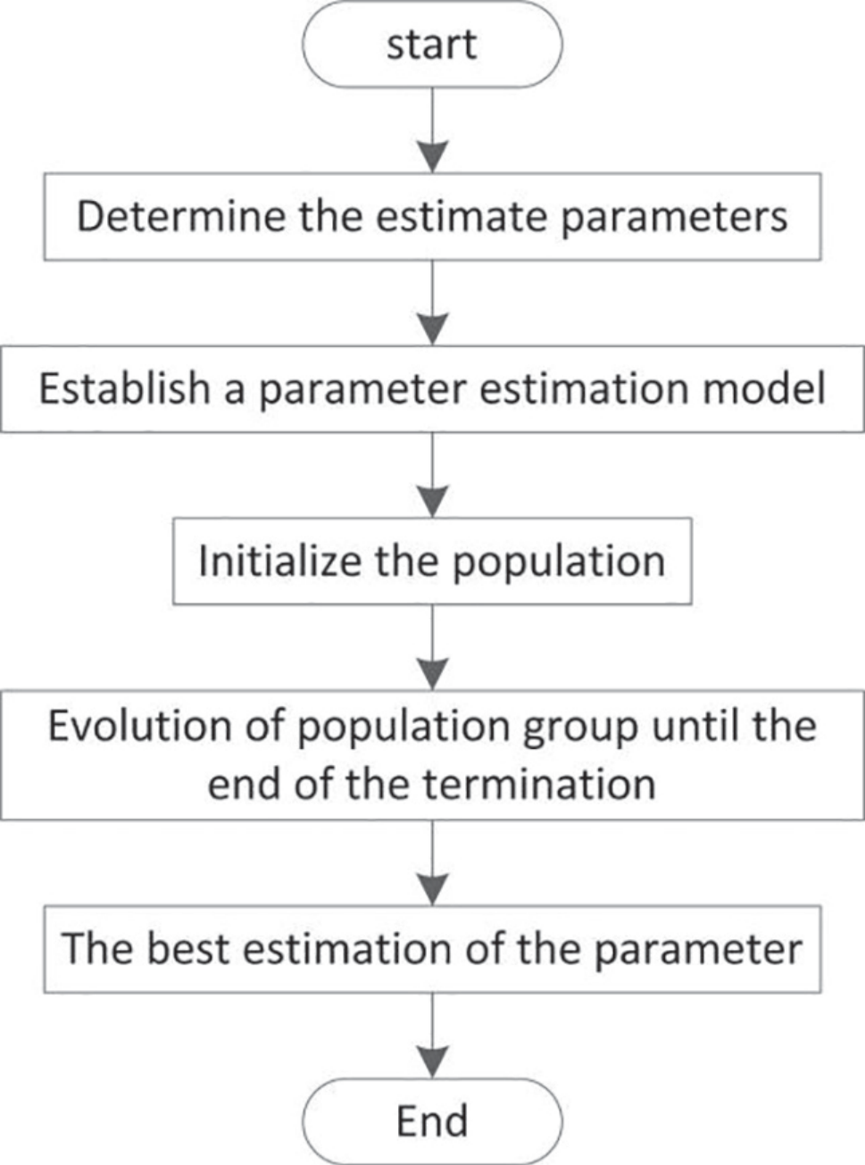
The objective function is taken as the log-likelihood function by the method in this paper, and it obtains corresponding constraint conditions of the parameters through the existing samples. The objective function, along with the constraint conditions, constitute the estimation model. Secondly, estimating the parameter value through an iterative process, and the accuracy of the parameter estimation value, is determined by the objective function. The larger the objective function is, the more accurate the estimated parameters are. Therefore, the optimal parameters are determined according to the parameters corresponding to the maximum value of the objective function. From this, the frame diagram of the estimated data mean and covariance matrix can be obtained, as shown in Fig. 2.
It is assumed that the data set U contains k variables of U1, U2,…, Uk and satisfies the k-dimensional normal distribution. The data set U contains missing data, recorded as U = (Uobs, Umis), Uobs is the data set with observed values, and Umis is the missing data set. For estimating parameters of the data set U, the proposed method uses a genetic algorithm. The parameters to be estimated are the mean and covariance matrix of the data. The upper limits and lower limits of the variable U1, U2,…, Uk are obtained from the data set Uobs, and are respectively recorded as [mini, maxi], i = 1, 2, …, k.
The log-likelihood function containing the mean and covariance matrix to be estimated is:
Where, ν = (ν1, ν2,…, νk) is the mean vector, representing the mean value of each variable; Σ = (ξpa) is the covariance matrix of the variable U1, U2,…, Uk; The initial values of ν and Σ are generally determined by the data set Uobs; ul represents the vector of the variable corresponding to the data record i = (1, 2, …, n), where n is the number of data records.
The accuracy of the estimated parameters is based on the size of the log-likelihood function. The problem is transformed into a single objective optimization problem to satisfy the g maximization of ν and Σ corresponding to all constraints. Its mathematical model is:
Where, mini, and maxi respectively mean the lower limits and upper limits of the i th variable. The constraint condition restricts that the estimated mean value of the variable must be between the maximum value and the minimum value of the variable. If the estimated mean value exceeds the range, it means that the estimated value is wrong and needs to be re-estimated.
(2) Population size setting and population iteration process
After determining the parameters to be estimated and the parameter estimation model, the parameter population should be randomly generated within the constraint conditions. The size of the population can be determined according to the data missing rate. In order to speed up the speed of obtaining the optimal solution, the first-generation population needs to include the mean and covariance matrix corresponding to the data set Uobs. After the initialization of an individual in the population, an adaptation function is needed to calculate the fitness of parameter individuals in the population to determine the degree of superiority and inferiority of the individual. The proposed method takes the objective function g(ν, Σ) as an adaptation function. When the value of the function is larger, the parameter is closer to the real value.
The population iteration process simulates the natural evolution law. According to the calculated individual fitness, some individuals with high fitness are reserved [33, 34]; at the same time, it can use crossover and mutation measures to evolve parameter individuals to achieve better parameter individuals. In the process of crossover and mutation, the two probability values corresponding to crossover probability Pc and mutation probability Pm will directly affect the evolutionary speed of the population, and are generally obtained through experience.
Where the cross evolution process is as follows: let Pc be the cross probability, the value range is (0, 1), and it is recommended to take 0.8. The parameter population contains n parameter individuals, and nPc parameter individuals are selected from the parameter population for cross-operation. Assuming that θ1, θ2, …, θn represents the parent of the parametric population, the two randomly selected parameters θr and θs form a cross pair, denoted as (θr, θs), r, s ∈ (1, 2, …, n) and i ≠ j. The crossover pair (θr, θs) is taken as an example to illustrate the process of crossover operation. A random number e is generated from the interval (0, 1), and ν is randomly selected from the set (1, 2, …, k). The crossover operation is performed on νrv and νsv in (θrv, θsv) to generate two descendants ν'rv and ν'rv , and new parameters θ'rv and θ'sv are obtained.
The evolution process of variation is as follows: let Pm be the variation probability, and the value range is (0, 1), and it is suggested to take 0.06. The parameter population contains n parameter individuals, and nPm parameter individuals are selected from the parameter population for cross-operation. Let θh be an individual in the parametric population, and the mean value contained in θh is (νh1, …, νhk). The random value γ within the range of (1, 2, …, k) is taken and mutated according to the above formula, then the mean value after mutation is (νi1, …, νiγ, …, νhk), and the parameter after mutation can be recorded as θh:
Where, random(∙) is a random function that generates a uniform distribution and generates a random number; Δ(z, x) = x[1 – ι(1–z/Z)χ]; ι ∈ [0, 1] is a random number, Z is the maximum variation algebra, z is the current variation algebra, and χ is the parameter that determines the degree of inconsistency.
The iteration termination condition of the parameter estimation of the proposed method is that the change range of the fitness function value corresponding to the optimal parameter is less than a small value β, i.e., |g*i – g*i–1| < β. Where,g*i is the value of the objective function corresponding to the optimal parameter while the iteration cycle is i times. Terminating the iteration and obtaining the optimal estimates the termination condition is satisfied. If satisfied, terminate the iteration to obtain the optimal estimation; If not, return to continue iterative optimization. It should be noted that the value range of β is (10-5, 10-3), and it is suggested that β is 10-4. Because the value of β is too small, the number of iterations will increase significantly, increasing the system overhead and iteration time, but the change of the objective function value is small. The value of β is too large, and the error of determined parameters is large, so the purpose of finding the optimal parameter individual is not realized.
Compared with the EM algorithm, a genetic algorithm is used to estimate the parameters of incomplete data, which expands the range of parameters to be estimated. In solving the data parameter problem, jumping out of local convergence and getting a better solution are easy, with better convergence ability and convergence speed.
(3) Missing data filling process
To improve the accuracy of the estimation, the proposed method uses the MCMC method to estimate missing data iteratively. The filling process is as follows:
1) Based on the mean vector, covariance matrix and data set Uobs, each missing data is estimated independently [35, 36], that is, the value of U (t+1) mis is obtained from the conditional distribution p(Umis | Uobs, θ(t));
2) According to the complete data set after filling, the posterior mean vector and covariance matrix of the simulation data, i.e. θ(t+1) is obtained from p(θ | Uobs, U (t+1) mis), which is put into step 1) and repeated.
The missing data of ecological environment symbiosis monitoring is filled by two steps (1) and (2) mutual iteration until the filled missing data and corresponding data parameters are no longer changed or the change range is within the allowable range. In other words, a Markov chain [(U(1), θ(1)), (U(2), θ(2)), … (U(t+1), θ(t+1))], is generated in the filling process, which converges on the p[(Umis, θ) | Uobs ]distribution. When the distribution is stable, Umis will be obtained to fill the missing data, and the final complete data set will be obtained.
Abnormal Monitoring Modeling of Symbiosis Monitoring Data in Ecological Environment
In previous section, the Markov chain Monte Carlo algorithm was used to estimate and fill in missing data, and the processed data was integrated into an ecological environment symbiosis monitoring dataset, which was used as the data foundation for abnormal monitoring modeling of ecological environment symbiosis monitoring data. The ecological environment symbiosis monitoring dataset was divided into extreme clusters, outlier clusters, and normal clusters. In each cluster, abnormal possibilities were assigned in different ways, and a time series diagram of abnormal possibilities was obtained that comprehensively considers independent variables and effect quantities. Based on this, an improved local anomaly coefficient calculation method was used to establish an abnormal monitoring model for ecological environment symbiosis monitoring data, in order to achieve the ultimate goal of high-quality monitoring of abnormal ecological environment symbiosis monitoring data.
The density clustering theory is a clustering method based on the density distribution of data points. In this method, areas with higher density may be divided into clusters, while areas with lower density may be considered as boundaries or noise between clusters. This clustering method does not rely on a pre-set number of clusters, but automatically determines the number and shape of clusters based on the actual distribution of data. The specific description of the advantages of density clustering theory in abnormal monitoring of ecological environment symbiosis monitoring data is as follows:
(1) Automatically determining the number and shape of clusters: Ecological environment data often has complex distribution patterns, making it difficult to pre-determine the number and shape of clusters. The density clustering theory can automatically determine the number and shape of clusters based on the actual distribution of data, thereby more accurately revealing the structure and function of ecosystems.
(2) Robustness to noise and outliers: In an ecological environment, data, noise, and outliers often exist. Traditional distance-based clustering methods may be sensitive to noise and outliers, while density clustering theory can better handle these noises and outliers by considering the density distribution of data points.
(3) Discovering clusters of arbitrary shapes: The distribution of species in ecosystems may exhibit various complex shapes, such as rings, bands, etc. The density clustering theory can discover clusters of arbitrary shapes, thus better reflecting the distribution patterns of species in ecosystems.
(4) Adapting to high-dimensional data: With the continuous development of monitoring technology, ecological environment data often includes multiple dimensions (such as temperature, humidity, lighting, etc.). Density clustering theory can adapt to high-dimensional data, thereby more comprehensively analyzing multiple factors in ecosystems.
(1) Local anomaly coefficient
Breuning proposed a local anomaly coefficient based on density. The coefficient is simple and intuitive, independent of the data distribution, and quantifies the abnormal degree of the symbiosis monitoring data points of the ecological environment by the ratio of the average local reachable density near the data points to the local reachable density of the data points.
After normalizing the effect quantity and independent variable of the symbiosis monitoring data of the ecological environment, the data set F is obtained. For the object point P and the object point A , the k-distance, k-neighborhood, reachable distance, local reachable density, and local anomaly coefficient of the object point P are defined as follows:
1) The distance of the k-th point closest to the point P is the k-distance fk(P) of the point k.
2) In the data set F, the point whose distance to the target point P is less than or equal to the k-distance of the point P is called the k-neighborhood Mk(P) of the point P:
Where, f(P, A) is the distance between point A and point P.
3) The maximum value of the distance from the target point A to the point P and the k-distance of the point P is called the reachable distance rd(P, A) from the point A to the point P:
4) The reciprocal of the average reachable distance of points in the neighborhood of point P is the local reachable density lrfk(P) of point P:
5) The ratio of the average local reachable density in the neighborhood of point P to the local reachable density of point P is the local anomaly coefficient LOFk(P) of point P:
From the above formula, if the LOF score of point P is around 1.0, it indicates that the local reachable density of point P is close to the average reachable density in the neighborhood; If the score is less than 1.0, it indicates that point P is located in a relatively dense area, the data points have similar properties, and the possibility that the points in the area are outliers is small; If the score is far greater than 1.0, it indicates that the data point P is far away from the points in the neighborhood, the properties of the data points are not similar, and the possibility of outliers is large. It should be noted that if the data set and k value are different, the threshold value is not 1.0 as the absolute standard.
(2) Improved local anomaly probability algorithm based on density clustering
Due to the complexity of the ecological environment, there are different degrees of deviation, different quantities, and different ranges of multi-modal outliers in the long-term monitoring data. The threshold needs to be further lowered to identify more outliers. As the threshold decreases, especially when it is lower than 2.0, more data points are judged as outliers, and misjudgment gradually appears. At this time, the LOF score of the data points fluctuates between 1.0 and 2.0, and the boundary between the outliers and other data points begins to blur, which is not conducive to the clustering of the symbiosis monitoring data of the ecological environment in the subsequent steps of the algorithm. Therefore, the reachable distance formula in the LOF algorithm is improved as follows:
Where, rν represents the improved reachable distance, which is called reachable variance; vark(P) is the variance of the distance from all points to point P in the k-neighborhood of point P; vark(P, A) is the variance of the distance between the k-neighborhood joining point A and point P of point P.
If the point A is far from the point P, the reachable distance is the actual distance between the two points. If the point A is close to the point P and within the neighborhood of the point P, the reachable distance is the k-distance of the point P. Taking out a smooth window, and the distance within the neighborhood of point P is set as a constant value. After exceeding the neighborhood range, the reachable distance increases linearly with the distance from point A. The distance is replaced with the variance of the distance, so that the linear increase becomes a nonlinear increase. The farther the distance is, the greater the value of rν is.
Therefore, the expression of local reachable density is improved as follows:
The expression of the local anomaly coefficient is improved as follows:
(3) Construction of abnormal monitoring model for ecological environment symbiosis monitoring data
Therefore, the local reachable density of the symbiosis monitoring data set in the ecological environment calculated according to the above formula can be divided into different data clusters. In the high-density area, the distance between data points is relatively close, the local reachable density is close to the average reachable density in the neighborhood, and the ILOF score is close to 1.0. It belongs to normal data points without abnormalities, which is called a normal cluster. In the transition area between the high-density and low-density areas, the distance between the data points is relatively long, and the local reachable density is different from the average reachable density in the neighborhood. The possibility that the data points are outliers gradually increases, which is called the outlier cluster. In the low-density area, the distance between data points increases significantly, and it can be determined as outlier points according to experience, which is called extreme cluster [37, 38]. The algorithm needs to find a suitable boundary point to distinguish the three clusters. Let the ILOF score sequence of the outlier cluster be (LOC1, LOC2, …, LOCt), then the average score LOCavg within the cluster is expressed as:
Where, t is the amount of data contained in the outlier cluster.
According to the characteristics of the ILOF algorithm based on density, when the value of t is small, the average value of ILOF scores in the low-density area is close to the ILOF scores of the data points, and the LOCavg in the abnormal cluster is close to 1.0. When the value of t increases, the distance between the data points in the cluster decreases and the density increases [39, 40]. The average ILOF score of the data points in the density transition area is greater than the ILOF score of the data points, and LOCavg in the abnormal cluster increases. The point increasing from 1.0 can be used as the boundary point between extreme clusters and outlier clusters. As the value of t continues to increase, the cluster gradually contains normal data points, and the ILOF score of normal data points is close to 1.0. Therefore, the mean value of ILOF scores in the data point field of the high-density area decreases, and LOCavg in the abnormal cluster decreases [41, 42]. The increasing or decreasing inflection point can be used as the dividing point between normal clusters and abnormal clusters. Normalizing the ILOF score sequence of the outlier cluster can obtain the quantification of the outlier anomaly probability.
To sum up, the separation of the ILOF algorithm from the normal cluster, outlier cluster, and extreme cluster constitutes an improved calculation method for local anomaly probability based on density clustering. The established anomaly monitoring model of symbiosis monitoring data in an ecological environment is shown in Fig. 3.
Results and Discussion
In order to verify the overall effectiveness of the research method for abnormal monitoring and modeling of symbiosis monitoring data in an ecological environment based on density clustering, it is necessary to carry out relevant tests. According to the research purpose of this study, it is assumed that compared with the comparison method, the proposed method has a higher accuracy rate of abnormal data monitoring, and shorter monitoring time of abnormal data which means higher efficiency, higher detection rate, and lower false detection rate.
The experimental parameters are set as follows: the operating system is Windows 10; the software is Linux; the simulation tool is Matlab 7.2; the programming language is VC; the integrated environment is Anaconda3; data processing in Python 3.8; the hardware memory is 8GB; the GPU is GeForce GTX 1080Ti.
By conducting on-site investigations and sampling, remote sensing technology, automatic monitoring stations, laboratory analysis, biological monitoring, and other methods, ecological environment symbiosis monitoring data can be obtained, and an ecological environment symbiosis monitoring dataset can be constructed. The data types in this dataset include physical data, chemical data, biological data, remote sensing data, behavioral data, time series data, etc. The specific introduction is as follows:
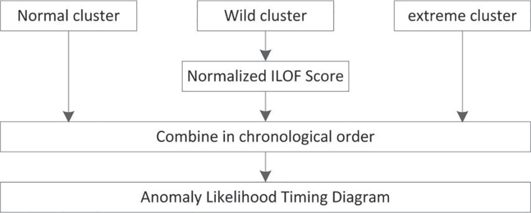
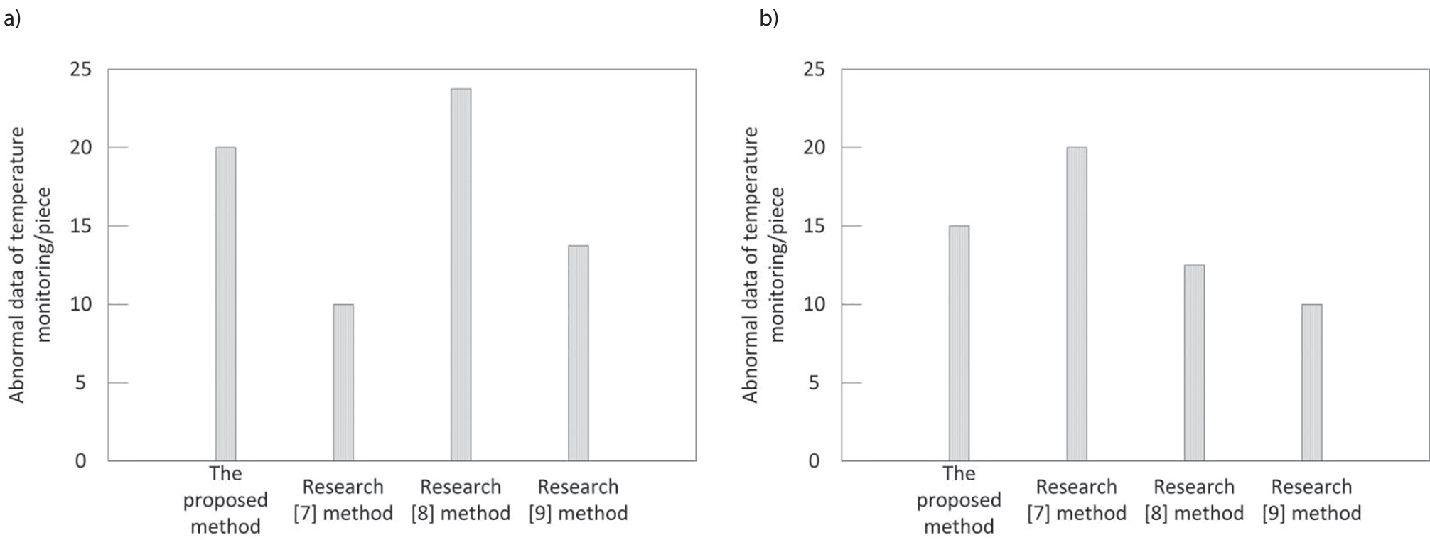
Fig. 4.
Data monitoring results of different methods. (a) Temperature monitoring data and monitoring results; (b) Humidity monitoring data and monitoring results.
Physical data: Such as temperature, humidity, light intensity, wind speed, rainfall, etc.
Chemical data: Such as soil pH value, nutrient content (nitrogen, phosphorus, potassium, etc.), dissolved oxygen in water, pH value, conductivity, pollutant concentration, etc.
Biological data: Such as species composition, biomass, population density, biodiversity index, niche width, etc.
Remote sensing data: Such as vegetation index (NDVI), land cover type, water distribution, etc.
Behavioral data: Such as animal migration paths, foraging behavior, reproductive behavior, etc.
Time series data: Records the changes of ecosystems over time, such as seasonal and interannual changes.
Set up an ecological environment symbiosis monitoring dataset consisting of 2000 temperature monitoring data and 2000 humidity monitoring data, including 20 temperature monitoring abnormal data and 15 humidity monitoring abnormal data. Now, the research method for abnormal monitoring modeling of symbiosis monitoring data in an ecological environment based on density clustering, the method of reference [7], the method of reference [8], and the method of reference [9] are adopted for carrying out data abnormal monitoring on the symbiosis monitoring data set of ecological environment. The monitoring results are shown in Fig. 4.
The analysis of the results in Fig. 4(a) shows that the proposed method can monitor 20 abnormal temperature data, the method in reference [7] can monitor 10 abnormal temperature data, and the method in reference [8] can monitor 24 abnormal temperature data. The method in reference [9] can monitor 13 abnormal temperature data, and only the abnormal temperature monitoring results of the proposed method are consistent with reality, indicating that the method has high monitoring accuracy. Analysis of the results in Fig. 4(b) shows that the proposed method can monitor 15 abnormal humidity data, the method in reference [7] can monitor 20 abnormal humidity data, and the method in research [8] can monitor 13 abnormal humidity data. The method in reference [9] can monitor 10 abnormal humidity data, and only the abnormal humidity monitoring results of the proposed method are consistent with reality, indicating that the method has high monitoring accuracy. Through comparison, it can be seen that when abnormal monitoring of temperature and humidity monitoring data is carried out using the proposed method, all abnormal data can be monitored, while other methods have the phenomenon of missing detection and false detection, because the proposed method cleans the data before monitoring, filters out the dirty data in the ecological environment symbiotic monitoring data, and fills in the missing data. The accuracy and integrity of the data are improved, and the accuracy of the data anomaly monitoring results is improved.
Taking the running time as an indicator, the monitoring efficiency of the proposed method, the method in reference [7], the method in reference [8], and the method in reference [9] are tested. The test results are listed in Table 1.
For different data volumes, the average operation time of the proposed method is 3.2375s, the average operation time of the method in reference [7] is 6.3625s, the average operation time of the method in reference [8] is 5.3s, and the average operation time of the method in reference [9] is 6.4625s. It can be found that the operation time of different methods increases with the increase in the data volume. Under the same data volume, the operation time of the proposed method is the least, indicating that the proposed method has high monitoring efficiency. The reason is that the proposed method uses the Markov chain Monte Carlo algorithm to estimate and fill the missing data on the basis of the optimal parameters. The ecological environment symbiotic monitoring data set was divided into extreme cluster, outlier cluster, and normal cluster, and the anomaly possibility was assigned to each cluster in different ways, and the anomaly possibility time series diagram considering independent variables and effect size was obtained. On this basis, an anomaly monitoring model of the ecological environment symbiotic monitoring data was established by using an improved local anomaly coefficient algorithm. Thus, the monitoring efficiency can be ensured to the maximum extent.
Table 1.
Operation time of different methods.
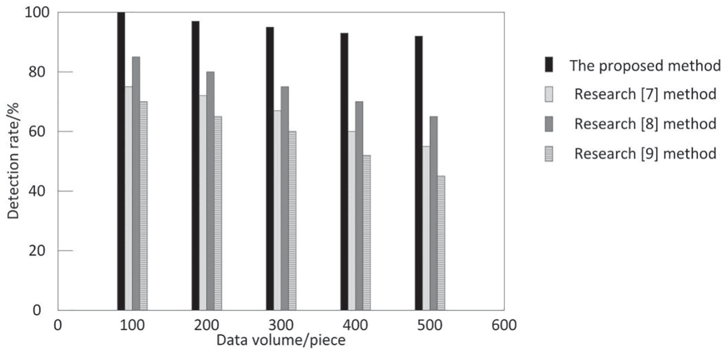
In order to further verify the effectiveness of the above methods, the rate of detection and false alarm are taken as indicators, and different methods are tested in the same test environment. The comparison results are shown in Fig. 5 and Fig. 6.
By analyzing the data in Fig. 5 and Fig. 6, it can be seen that with the increase in data volume, the detection rate and false detection rate of the four methods show a decreasing and increasing trend, respectively. Among them, the detection rate of the proposed method is always above 90%, the detection rate of the method in reference [7] is between 56% and 74%, and the detection rate of the method in reference [8] is between 66% and 85%. The detection rate of the method in reference [8] was between 55% and 70%. In the process of false detection rate testing, the false detection rate of the proposed method is always lower than 7%, the false detection rate of the method in reference [7] is between 7% and 13%, and the false detection rate of the method in reference [8] is between 8% and 17%. The false detection rate of the method in reference [9] is between 5% and 15%. Compared with the test results of the other three methods, it is found that the proposed method has a high detection rate and a low false detection rate. The high detection rate means that the proposed method can accurately identify abnormal phenomena in the ecological environment, which is crucial for timely detection and treatment of environmental problems. The low false detection rate means that the proposed method does not frequently cause false alarms or issue unnecessary alarms, thus reducing operator interference and unnecessary waste of resources. This reliability ensures that the output information of the system has high reliability, indicating that the abnormal monitoring of the ecological environment symbiosis monitoring data has a good monitoring performance.
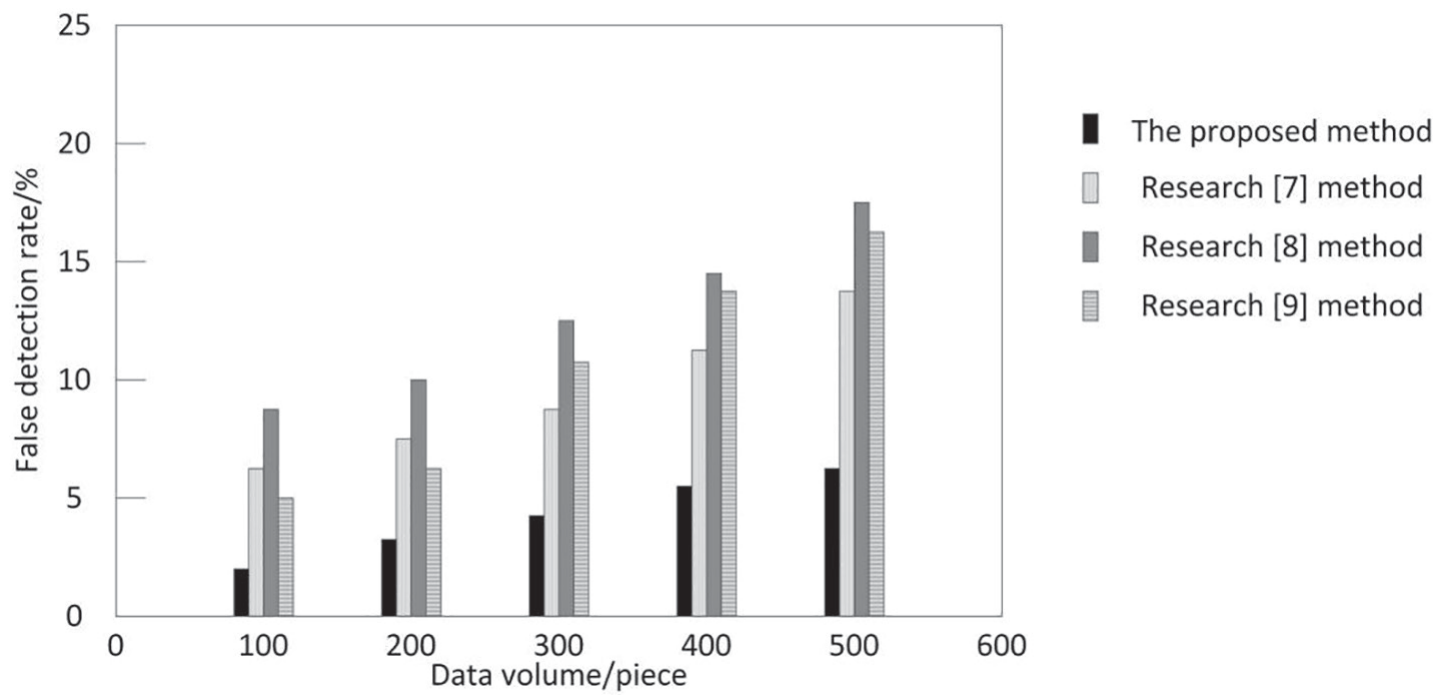
Table 2.
F1 score comparison results.
Table 3.
Comparison results of false positive rates.
On this basis, two indicators, F1 score and false positive rate, were selected to verify the application effects of different methods. The specific results are shown in Tables 2 and 3.
According to the analysis of Table 2, the mean F1 score of the proposed method is 0.94, the mean F1 score of the method in reference [7] is 0.77, the mean F1 score of the method in reference [8] is 0.69, and the mean F1 score of the method in reference [9] is 0.68. After comparison, it can be seen that the proposed method has the highest mean F1 score, indicating that the ecological environment symbiosis monitoring data anomaly monitoring effect of this method is good.
According to the analysis of Table 3, the mean false positive rate of the proposed method is 0.24%, the mean false positive rate of the method in reference [7] is 3.19%, the mean false positive rate of the method in reference [8] is 14.32%, and the mean false positive rate of the method in reference [9] is 10.21%. A low false positive rate means that the error in the abnormal detection results of the ecological environment symbiosis monitoring data of the proposed method is low, which can improve the overall monitoring accuracy.
Limitations and Directions for Improvement
The proposed method applies the improved algorithm in data cleaning and missing data filling to improve the convergence speed and level, so as to improve the accuracy and efficiency of abnormal monitoring of ecological environment symbiosis monitoring data. However, the designed abnormal data monitoring model does not have the specific refinement of ecological environment parameters and the weight evaluation of ecological environment parameters. Ecological environment parameters include geology, soil, hydrology, climate, plants, wild animals, etc. In order to apply the designed abnormal data monitoring algorithm to the ecological environment symbiosis monitoring, the classification of experimental data will be refined in the next step to verify whether the algorithm can improve the reliability of the ecological environment symbiosis monitoring data and reflect the improvement of the ecological environment.
Conclusions
The symbiosis monitoring data of the ecological environment is an important basis for analyz ing and evaluating the ecological environment. However, the symbiosis monitoring data of the ecological environment is usually affected by the structure, environment, and time cycle, resulting in abnormal monitoring data. It is necessary to carry out abnormal monitoring research of symbiosis monitoring data in the ecological environment. At present, the abnormal monitoring methods for symbiosis monitoring data of ecological environment have the problems of low monitoring accuracy, low monitoring efficiency, low detection rate, and high false detection rate. In view of these problems, a research method of abnormal monitoring and modeling of symbiosis monitoring data in the ecological environment based on density clustering is proposed. This method first cleans the ecological environment symbiosis data and fills in the missing values. On this basis, an improved local anomaly probability algorithm based on density clustering is used to establish the anomaly monitoring model of the symbiosis monitoring data in the ecological environment. The experimental results imply that the method in this paper can increase the monitoring accuracy and efficiency, improve the rate of detection, and reduce the rate of false detection. It is hoped that the proposed method can provide a valuable reference for the abnormal monitoring of symbiosis monitoring data of the ecological environment. Different data sets have different characteristics, such as data distribution, dimension, noise level, etc. These characteristics will directly affect the effect of the anomaly monitoring method based on density clustering. For example, in high-dimensional data sets, traditional distance measurement methods may fail due to the “dimensional disaster” problem, resulting in poor anomaly detection. Therefore, when the method is applied to different data sets, it needs to be adjusted and optimized according to the characteristics of the data sets. Different environmental backgrounds have different requirements for anomaly monitoring methods. For example, in air pollution monitoring, more attention may be paid to data points where concentrations change dramatically over a short period of time; in water quality monitoring, however, more attention may be paid to data points with persistent anomalies over time. Therefore, when the anomaly monitoring method based on density clustering is applied to different environmental backgrounds, it needs to be customized and adjusted according to specific needs. When the proposed method is used to carry out abnormal monitoring of temperature and humidity monitoring data, all abnormal data can be monitored. The average operation time of the proposed method is 3.2375s, the detection rate is always above 90%, and the false detection rate is always lower than 7%. These data are obtained by repeated experiments on multiple data sets and are relative according to indicators. Therefore, this method has a strong universality. This study may provide new tools and methods for ecosystem management, helping decision-makers better understand and predict the dynamic changes of ecosystems, thereby formulating more effective management measures. However, this method also has some limitations. For example, a genetic algorithm, as an optimization algorithm that simulates natural evolution, usually has high computational complexity. When processing large-scale ecological environment data, it may require a lot of computing resources and time, which will affect the real-time efficiency of data anomaly monitoring. Moreover, the estimation of missing data is usually accompanied by uncertainty, which may spread to the subsequent anomaly monitoring process, thus affecting the reliability of monitoring results. In the future, these limitations should be fully considered and corresponding measures should be taken to reduce their impact on anomaly monitoring results. For example, the accuracy and reliability of anomaly monitoring can be improved by optimizing genetic algorithm parameters, selecting appropriate missing data estimation methods, and improving the algorithm based on density clustering.