

Introduction
Ecosystem services (ES) are crucial for maintaining a delicate balance between environmental sustainability and economic prosperity [1-3]. These services, quantified as ecosystem service values (ESV), encompass a broad array of benefits derived by humanity from ecosystems [4]. In the 21st century, marked by globalization and resource depletion, the importance of ES has significantly increased [5]. Basin ecosystems, especially those in China, play dual roles as economic engines and ecological barriers, highlighting their indispensable nature [6, 7]. The concept of ESV [8, 9], which is influenced by socioeconomic and ecological factors, varies across basins due to human activities [7, 10]. Understanding these variations is vital for developing effective and contextually appropriate conservation and development strategies [11]. China’s rapid urbanization has led to a notable decline in ESV, necessitating a comprehensive spatial analysis [12]. From a basin-centric perspective, carefully examining how ESV respond to land use change patterns and protection measures is essential for enhancing ecological conservation and promoting high-quality development.
A detailed understanding of the spatial and temporal diversity of ESV is instrumental in supporting regional sustainable development and ecosystem management. As a primary determinant of ESV, land use change leads to notable fluctuations, particularly in the context of urbanization [13, 14]. Quantifying the complex relationship between ES and land use change is essential for protecting multiple ES [15, 16]. ESs are complex systems where services and values are intertwined, resulting in trade-offs and synergies [17, 18]. On the one hand, further research into the tradeoffs and synergies inherent in ES is vital for advancing sustainable development and ensuring the long-term viability of ecosystems. On the other hand, the majority of studies on ESs have concentrated on cities [19], regions [8], or single basins [20]. Studying ESs across different basins within the same region offers a precise reflection of the biophysical characteristics of the area [21]. This provides a distinct advantage in addressing the disconnect between ecological processes and human management frameworks. This cross-basin analysis underscores the value and significance of understanding ecosystem interdependencies at the scale of the same administrative boundary, fostering more sustainable and holistic management strategies.
Since the advent of the ESV concept, quantifying it has been pivotal in ecological economics [22]. While studies have analyzed ESV changes due to land use change, they frequently neglect spatial interactions [23, 24]. Researchers have gradually explored spatial effects, highlighting the importance of considering spatial dimensions in ESV assessments [25, 26]. Despite attempts to assess ESV variations across regions, these studies focused mainly on isolated basins or singular regions [27, 28]. In complex ecosystems spanning multiple basins, ESV discrepancies between regions can be substantial. Thus, exploring methodologies to harness these differences and formulating tailored ecological management strategies are crucial for future research. To adapt the globally developed equivalent factor table to China’s terrestrial ecosystem, a survey was conducted among 500 Chinese ecologists, resulting in subsequent modifications [29, 30]. Using this adapted table, the present study evaluates the spatiotemporal evolution of ESVs across various basins in Henan Province (HNP) [31, 32]. In addition to quantifying the impacts of land use on ESVs, this study identifies hot and cold spots of ESV changes and elucidates the underlying mechanisms driving these spatial patterns. This basin-centric approach is vital for promoting harmonious natural and economic development, enhancing ecological protection, and guiding strategies for environmental protection and sustainable economic growth [33]. Considering the multitude of ES and their intricate interrelationships across different basins is imperative, rather than prioritizing isolated basins for ecological management. Analytical methods, such as one-way analysis of variance (ANOVA) and correspondence analysis, have proven effective in assessing ESV across diverse basins [34, 35]. Differential evaluations of ESV across ecological subsystems and the distinctive attributes of ESV at the basin scale deepen our understanding of the developmental patterns of service values among regional ecosystems. This enhanced understanding bolsters basin-level ecosystem protection efforts by revealing evolutionary trends in service value patterns. In conclusion, examining ESV from a basin perspective enhances our comprehension of ES dynamics and reinforces our capacity to manage these services sustainably across various regional contexts. This holistic approach is essential for ensuring the long-term preservation and sustainable utilization of ecosystem services.
The HNP, a prominent grain-producing region in China [36], spans four river basins: the HUB, YEB, YZB, and HAB. These basins display considerable variation in their provision of ESs, shaped by climate and land use patterns. The HUB, an economic and population hub, also serves as a climate transition zone [37], highlighting its dual economic and ecological significance. The YEB acts as a crucial ecological barrier prioritized for national preservation and sustainability [38]. Conversely, YZB is characterized by ecological fragility, resource constraints, and uneven economic development [39], necessitating prudent management. HAB faces China’s most severe water scarcity, underscoring the need for effective water management [40]. National policies, such as “returning farmland to forests” and the South-to-North Water Diversion Project, have enhanced HNP ecological conditions and land management [41]. Each river basin presents unique challenges and benefits from these policies. However, studies lack a basin-level understanding of ES and sustainable management interactions. Understanding these interactions is vital for crafting effective regional ecological conservation strategies, achieving long-term objectives, and promoting environmentally sustainable, economically viable development [42].
This study examines the heterogeneous spatial impacts of land use on the ESV in four HNP basins, addressing regional coordination and management. The objectives of this study include exploring ES spatiotemporal changes, coordination, trade-offs, and ESV disparities and assessing their implications for sustainable ecosystem management. By rigorously examining the land use ESV interplay, this study advances ecological economics and informs policies for sustainable development, guiding effective conservation and management strategies to ensure basin ecosystem viability and resilience.
Materials and Methodologies
Study Area
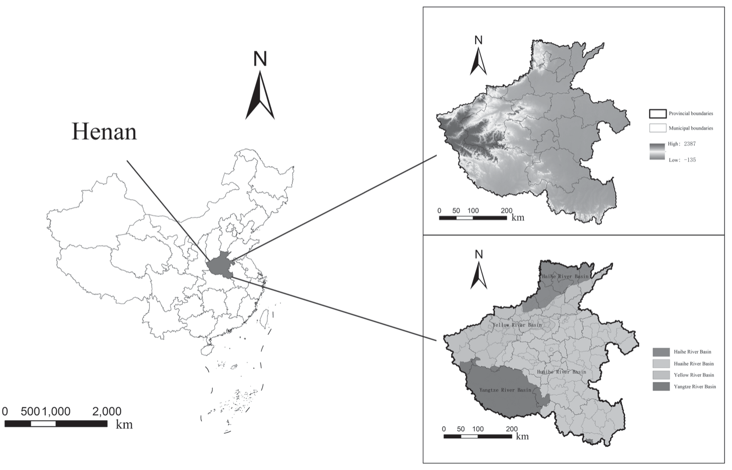
The HNP (110°21′-116°39′E, 31°23′-36°22′N), situated in east-central China along the middle and lower reaches of the Yellow River, spans an area of approximately 167,000 km² (Fig. 1). The topography of the province is diverse and is characterized by elevated terrains in the west and lower plains in the east. Plains and hilly mountains make up 55.7% and 44.3% of the total area of the province, respectively. Four major river systems traverse the HNP: the Yellow River, the Huai River, the Hai River, and the Yangtze River. The climate transitions from a warm temperate zone in the north to a subtropical zone in the south, shaped by a continental monsoon climate with pronounced seasons, simultaneous rain and heat periods, diverse ecosystems, and frequent climatic extremes. In the past decade, the annual average temperature has fluctuated between 12.9ºC and 16.5ºC, with the annual precipitation ranging from 464.2 mm to 1193.2 mm. The annual average sunshine duration falls between 1505.9 hours and 2230.7 hours, promoting favorable conditions for varied crop growth. The HNP is composed of four distinct basins, HUB, YEB, YEB, and HAB, each molded by unique climatic conditions, natural resources, and geographical positions, resulting in diverse developmental trajectories. Changes in land use patterns within these basins have profoundly influenced local ecosystems.
Evaluation Framework
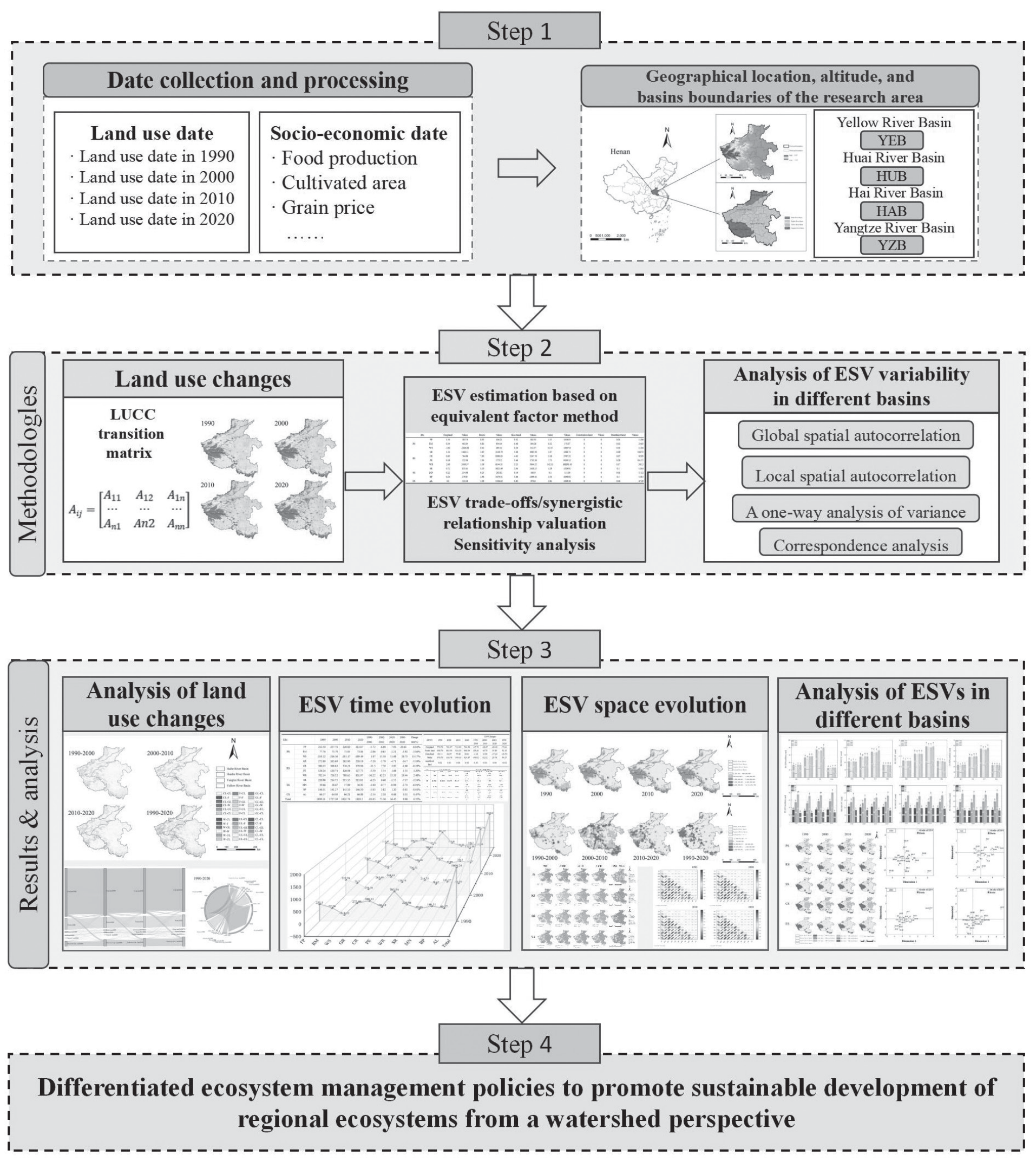
This study constructed a comprehensive evaluation framework for examining the variations in land use and ESV across distinct basins in HNP (Fig. 2). Relevant data, including land use records from 1990- 2020 and socioeconomic indicators such as grain output, grain prices, and planted areas, were collected. A delineation of four basin districts in Henan Province – YEB, YZB, HUB, and HAB – was established. The evaluation framework subsequently incorporated multiple methodological approaches. First, the land use transfer matrix was utilized to assess the dynamics of land use transitions within HNP. The equivalent factor method was employed to quantify ESVs across the four basins, thereby facilitating a comprehensive assessment of the trade-offs and synergies among ES. This study then deployed spatial autocorrelation analysis, hot spot analysis, and one-way ANOVA to investigate spatial clustering characteristics, hot spot and cold spot distributions, and significant variations in ESVs among different basin districts. Specifically, spatial autocorrelation analysis was used to examine the spatial clustering tendencies of ESVs within various basin districts, whereas hot spot analysis pinpointed the spatial aggregation patterns of ESV hot spots and cold spots across distinct functional zones. Then, by leveraging correspondence analysis, we evaluated distinct classes of ESs across the four basins to reveal disparities in ESVs across the regions. Finally, customized ecosystem management strategies have been proposed for each basin to augment the capacity for ES provision and promote sustainable ecosystem development across HNP.
Methods
Land Use Changes
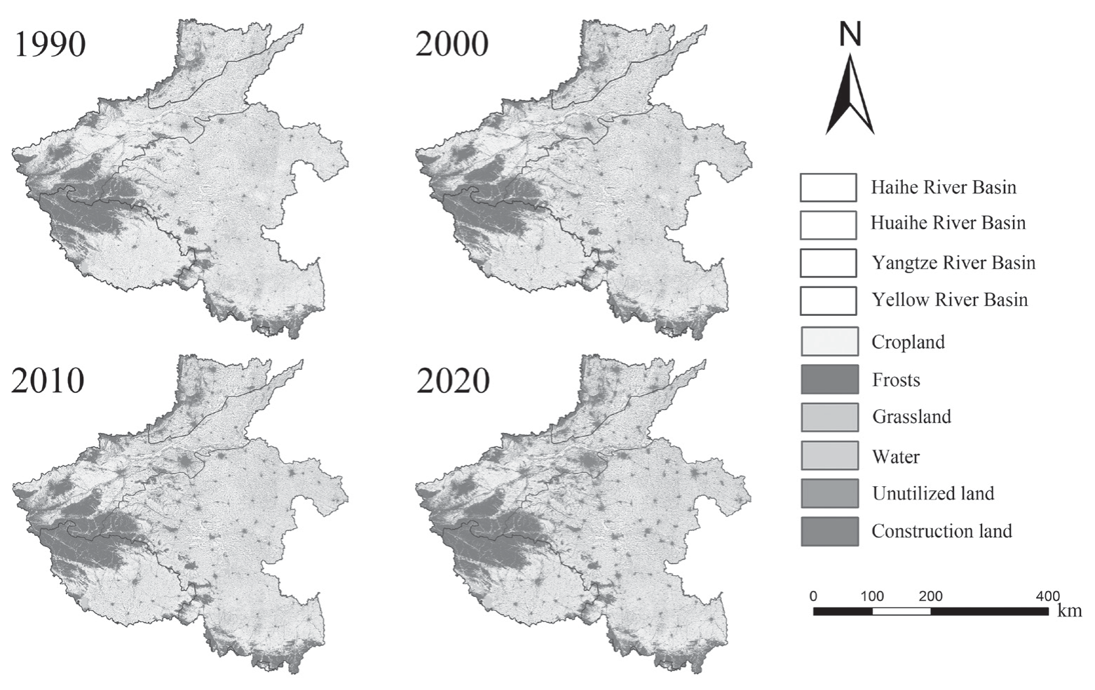
Within the study area, land use was classified into six categories: cropland, forest, grassland, water, construction land, and unused land (Fig. 3). The dynamics of each land use type are intended to directly mirror alterations in their quantity over time [43]. This is accomplished by quantitatively detailing the area transition of each specific land use type within the study period.
The land use transition matrix illustrates the quantitative relationships between the conversions of various land use types across two distinct time periods [44]. It effectively captures the magnitude and direction of these transitions within the study area. In this study, which relies on land use data from the HNP, alterations from 1990--2020 were analyzed via the ArcGIS tool. This analytical methodology offers a comprehensive appraisal of how land use patterns have transformed over the study period.
where n denotes the total number of land use types in the study area, n = 7, and Aij is the area transferred from land use type i to land use type j.
Calculation of ESV Per Unit Area
As depicted in Table 1, this study adopted the equivalent value of ESV per unit area, which was specifically developed for China [32, 31]. The ESs were categorized into provisioning services (PS) encompassing food production (FP), raw material (RM) and water supply (WS); regulating services (RS) comprising gas regulation (GR), climate regulation (CR), water regulation (WR) and purification of the environment (PE); supporting services (SS) involving soil retention (SR), maintaining nutrient cycling (MN), and biodiversity protection (BP); and cultural services (CS), including the aesthetic landscape (AL). The economic value of a single equivalent factor of ESV equates to 1/7 of the average market value of food production per unit area derived from cultivated land [31].
Consequently, the study revised the economic value of a single equivalent factor of ESV per unit area, correcting it on the basis of the basic data of grain production, grain prices, and cultivated area of three major grain crops (wheat, corn, and rice) within HNP. The formula is as follows:
where Ea is the economic value of the FP per unit area from cultivated land (CNY/ha); g is the main food crop type; m is the number of food crops; ag, pg, and qg are the cultivated area, grain price, and FP of food crops, respectively; and M is the total area of food crops.
In this study, the average value of Ea was determined to be 1183.5 yuan hm-2 a-1. The value coefficients for each ES in the HNP were calculated via the 1990-2020 Henan Provincial Statistical Yearbook and the National Compendium of Agricultural Product Costs and included the sown area and yield of rice, wheat and maize, as well as the national average selling price for the main products per 50 kg during different years within the HNP.
The ESV equivalent per unit area of land use type was calculated for the ecosystem service types as follows:
where VCik is the modified ESV per unit area of an ecosystem of the ith ES provided by land use type k, and eik is the equivalent factor.
According to the VC results, individual and total ESV were calculated as follows:
where ESVi and ESV are the individual ESV and total ESV, respectively, and Ak is the area of land use type k.
ESV Trade-Off/ Synergy Evaluation
We utilized 10 km × 10 km grid cells as the evaluation units to assess ESV for each service across four temporal points: 1990, 2000, 2010, and 2020. Subsequently, correlation analysis was conducted, starting with a Pearson correlation coefficient (r) greater than zero (P<0.05), indicating synergistic relationships between different ESs, with a stronger coefficient reflecting a more robust synergistic interaction [45]. Conversely, a negative correlation coefficient (r<0, P<0.05) represented a trade-off among the services, where a lower coefficient indicated a more significant trade-off. A correlation coefficient of zero (r = 0, P<0.05) suggested the absence of a linear relationship between the two services.
Sensitivity Analysis
The sensitivity of the ESV in HNP was assessed via the sensitivity index to evaluate the validity and reliability of selected ESV coefficients in the study area [33]. A conservation sensitivity (CS) value exceeding 1 indicates ESV resilience to fluctuations in the valuation coefficient (VC), confirming the high reliability of the results. Conversely, a CS value below 1 implies that ESV is sensitive to changes in VC, underscoring the necessity for more reasonable ESV coefficients. Adjustments were made to the ESV coefficients of different land use types by 50% to calculate CS, thereby emphasizing ESV sensitivity to VC:
where ESVi is the ESV of lands in the study area during the early stage, ESVj is the adjusted ESV in HNP, and VCik and VCjk are ESV coefficients of land use type k before and after adjustment.
Spatial Autocorrelation Analysis
The first law of geography posits that objects in geographic space exhibit relationships in which closeness promotes enhanced correlation relative to more distant entities. Spatial autocorrelation serves as a spatial data analysis method to assess the correlation between a location in space and its neighboring locations, gauging the extent of this correlation [46]. This method encompasses both global spatial autocorrelation and local spatial autocorrelation. In this study, global spatial autocorrelation was employed to capture the spatial clustering characteristics of ESV in HNP. The equation used is detailed as follows [47, 48]:
Table 1.
Equivalent factors and values of ESV per unit area for various LUCC types in HNP.
where I is the global spatial autocorrelation index and wji is the spatial adjacency weight between counties i and j. I > 0 indicates a positive spatial correlation, I = 0 indicates no spatial correlation, and I<0 indicates a negative spatial correlation. Larger values indicate greater spatial clustering of ESVs.
Hotspot Analysis
At a small scale, local autocorrelation differentiates hotspots from coldspots, specifically identifying spatial clusters of statistically significant high (hot spots) and low (cold spots) values of ESV [49, 50]. Following iterative testing, a 10 × 10 km fishnet grid was determined as the optimal scheme for this division. The Zonal Statistics tool in ArcGIS 10.8 was then applied to calculate the average ESV for each square. Finally, the Getis-Ord GI* tool in ArcGIS 10.8 was used to identify ESV hot spots and cold spots across diverse functional areas. The significance testing of Getis-Ord G* values (Gu*) was conducted via z scores and p values, with values deemed statistically significant at p = 0.05 (95% confidence level). The specific calculation methodologies are detailed as follows:
where xv is the ESV for grid v, wuv is the spatial weight between grid u and grid v, and t is the total number of grids.
One-way Analysis of Variance
The statistical significance of ESV differences is assessed through one-way analysis of variance (ANOVA), followed by the least significant difference test (with a significance level of p<0.05) [51]. Consequently, one-way ANOVA was used to scrutinize ESV variations across different basins. The Zonal Statistics tool in ArcGIS 10.8 was used to derive ESV values for each basin. One-way ANOVA was conducted via SPSS 26.0 statistical software.
Correspondence Analysis
CA serves as a graphical method for exploring the relationships between samples (rows) and variables (columns) in a low-dimensional space [34]. Central to performing CA is the use of a data transformation method that converts the original data matrix, consisting of M samples and N variables, into another matrix. The crux of executing CA is the utilization of a data transformation method, which transmutes the original data matrix comprising M samples and N variables into a different matrix. This transformation process is executed as follows:
In this study, the variation in ESV throughout the study area from 1990-2020 was categorized into five grades (I, II, III, IV, and V) via the arithmetic discontinuity method in conjunction with the ArcGIS Spatial Analyst module. The distribution levels of the four types of ES and the four basins were treated as samples, with their corresponding areas acting as variables. This investigation sought to ascertain the correspondence between four basins and 20 levels of ESV alteration (consisting of four ES types, each classified into five levels).
Results
Spatiotemporal Dynamic Analysis of Land Use
As shown in Fig. 4, the spatiotemporal dynamics of land use were illustrated in HNP across various years. The study area encompasses a variety of land types, including croplands, forests, grasslands, construction lands, waters, and unused lands. Croplands, construction lands, and forests exhibit a clustered distribution, whereas water and grasslands are dispersed across the region. Croplands, consisting of both dry lands and rice paddies, span from the northern to the southern parts of the HNP. Over the years, construction land, which has been predominantly concentrated in the HUB, has shown a gradual decline. Concurrently, substantial conversions of construction lands have been observed in YEB, which includes Zhengzhou and Luoyang. Forests and grasslands are located primarily in the Qinling Mountains at the confluence of three major river basins, the southern region of the YZB, and the Taihang Mountains, where HAB and YEB meet. The spatial distribution of construction lands closely mirrors that of croplands, which are predominantly clustered around urban areas within each basin. Waters were sporadically distributed throughout the HUB and YZB. This study integrates the spatial patterns of land use in HNP, highlighting notable shifts in land use over the years, while elaborating on the distribution traits of various land use types across disparate geographic regions.
As illustrated in Fig. 5, significant transformations were recorded across various land use categories within the HNP. Croplands stand out as the predominant type, encompassing more than 60% of the total area. Cropland, forests, and construction land consistently occupy the top ranks in terms of land use. Notably, unused land has undergone a more pronounced reduction, whereas construction land has exhibited a substantially higher growth rate. When analyzed from a basin-specific perspective, the HUB basin experienced a gradual decline in cropland, which primarily transitioned into construction land, with some areas also converting to forestland between 1990 and 2020. A notable surge in construction land was observed during this period. In the YEB, both construction land and forests expanded, whereas cropland contracted significantly. The amount of water initially decreased but subsequently increased, and the amount of grassland initially increased but then decreased. The YZB exhibited relatively stable overall trends, with construction land and grassland showing annual increases. Water bodies initially decreased but later increased. Between 2010 and 2020, prominent shifts included a reduction in cropland and an increase in forestland. In HAB, cropland also decreased, primarily transforming into construction land, whereas grassland initially expanded and then contracted.
Table 2 reveals that from 1990-2020, the annual average rates of land use change were -1.47% for unused land and 3.06% for construction land. These alterations reflect the impacts of urbanization, economic development, agricultural land structure adjustments, and unsustainable land use practices. During the rapid economic growth of the 1990s, extensive development activities led to the conversion of significant grassland areas into construction land. Throughout the past three decades, the forest area has remained relatively stable, experiencing a minor decline followed by moderate recovery by 2020, attributed to governmental initiatives aimed at protecting forest ecosystems. Similarly, grasslands decreased from 1990-2020, following a trend comparable to that of construction land. Conversely, water mirrored the fluctuation pattern observed in forests, initially decreasing from 1990-2000 by 260.95 km², followed by an increase of 523.1 km² from 2000-2020. These shifts underscore the influences of climate dynamics and ecological restoration efforts.
Spatiotemporal Evolution of ESV
Temporal Evolution of ESV
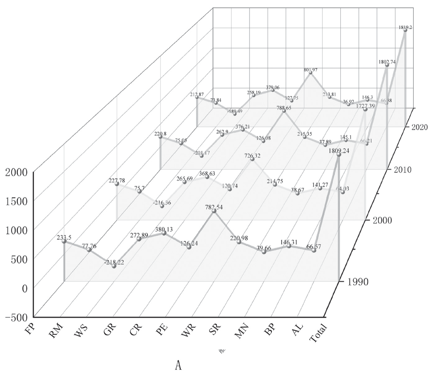
By utilizing the equivalent values of land use, socioeconomic factors, and ecosystem services per unit area (Table 1), the ESV of HNP from 1990-2020 can be computed via Equation 3. As depicted in Fig. 6, from 1990-2020, the ESV within the region initially decreased but then subsequently increased. Overall, the aggregate value of ESs increased from 1809.24 billion CNY to 1819.2 billion CNY, an increase of 0.55%. At the ES classification level (Table 3), the PS, RS, SS, and CS values presented growth rates of -4.85%, 0.84%, -1.75%, and 1.34%, respectively. From 1990-2000, the PS, RS, SS, and CS values decreased by -6.14%, -4.94%, -2.83%, and -3.52%, respectively. Between 1990 and 2020, all aspects increased, with the exception of SS, which demonstrated a minor decrease of 0.66% from 2000-2010, whereas all the other aspects displayed an increasing trend. Among them, RS held the largest proportion, and CS held the smallest proportion. In the computation and statistical results of the secondary classification of ESVs, only the ESVs of water SS, environmental purification, and hydrological RS increased, with growth rates of 13.17%, 1.2%, and 2.48%, respectively. The remaining nine ESs exhibited negative value growth, with FP (-8.84%) declining the fastest and biodiversity services (-0.01%) declining the slowest; the growth rates of RM, GR, CR, SC, MN, and AL were -5.04%, -5.39%, -0.28%, -3.24%, -6.91%, 0.47%, and -20.18%, respectively.
Fig. 4.
Land use changes in four watersheds in Henan from 1990 to 2020. (CL stands for Cropland, F for Frosts, GL for Grassland, W for Water, UL for Unused Lands, and CL for Construction Land)
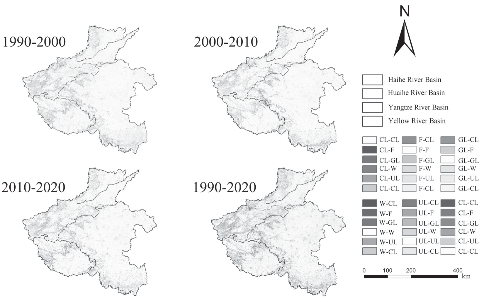
Fig. 5.
Changes in different land use types, 1990-2000, 2000-2010, 2010-2020 and 1990-2020, a denotes land use in HNP, b denotes land use in HUB, c denotes land use in YEB, d denotes land use in YZB, e denotes land use in HAB.
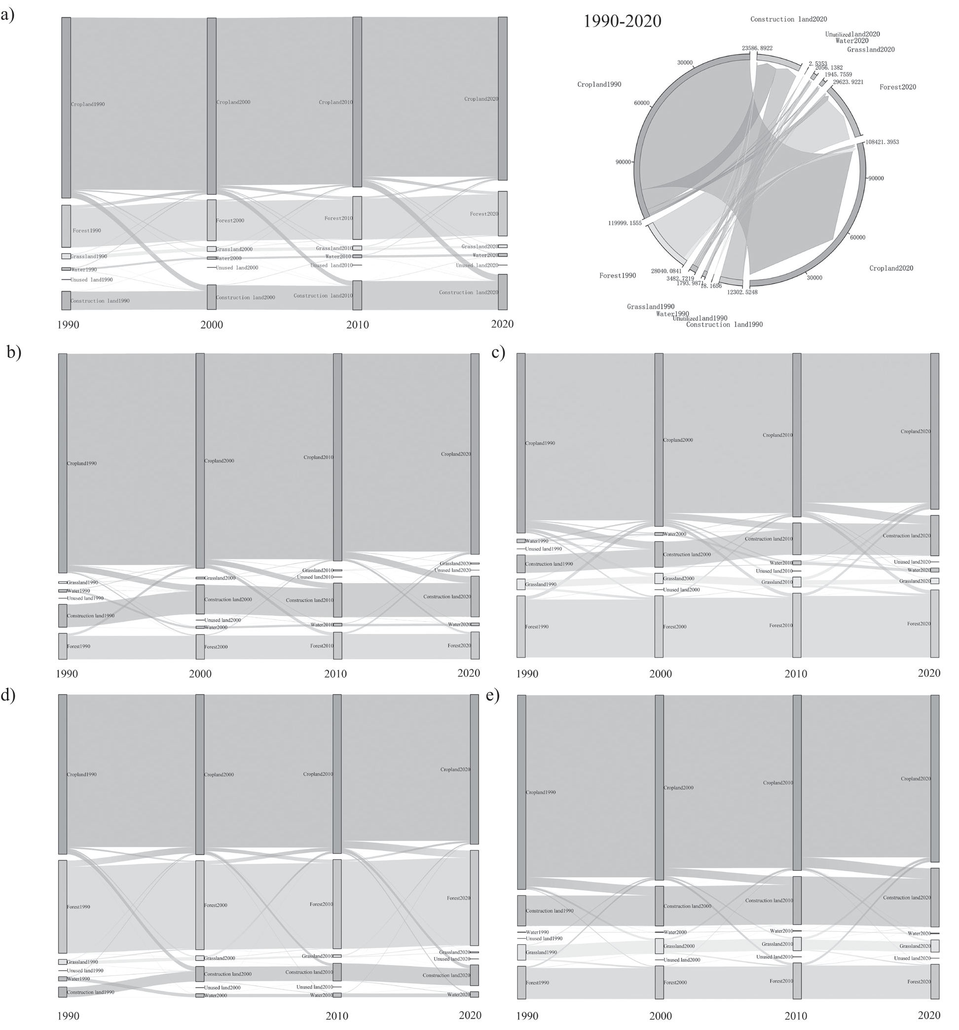
Table 2.
Characteristics of LUCC structure in HNP, 1990-2020.
Table 3.
Changes in ESV at the level of Henan 1990-2020.
With respect to the ESV produced by each land use type (Table 4), forests contributed the highest ESV, followed by cropland and water, whereas the remaining land use types generated comparatively low overall ESV. Cropland, grassland, and unused land exhibited consistent annual reductions of -75.23 billion CNY, -30.50 billion CNY, and -0.02 billion CNY, respectively. The proportion of ESV contributed by forests to the total ESV consistently surpassed 45%. However, from 1990-2000, the total ESV provided by each land type demonstrated a downward trend due to the expansion of urbanization; in particular, forests and water decreased by nearly 25.26 and 53.92 billion CNY, respectively. Under the influence of environmental conservation policies, the proportion of ESVs contributed by both forests and water demonstrated a growing trend from 2000-2020. Specifically, they increased by 51.33 billion CNY and 54.17 billion CNY. Forests and water stand as the primary land use types that provide ecological products or services for humans in these functional areas.
Spatial Evolution of ESV
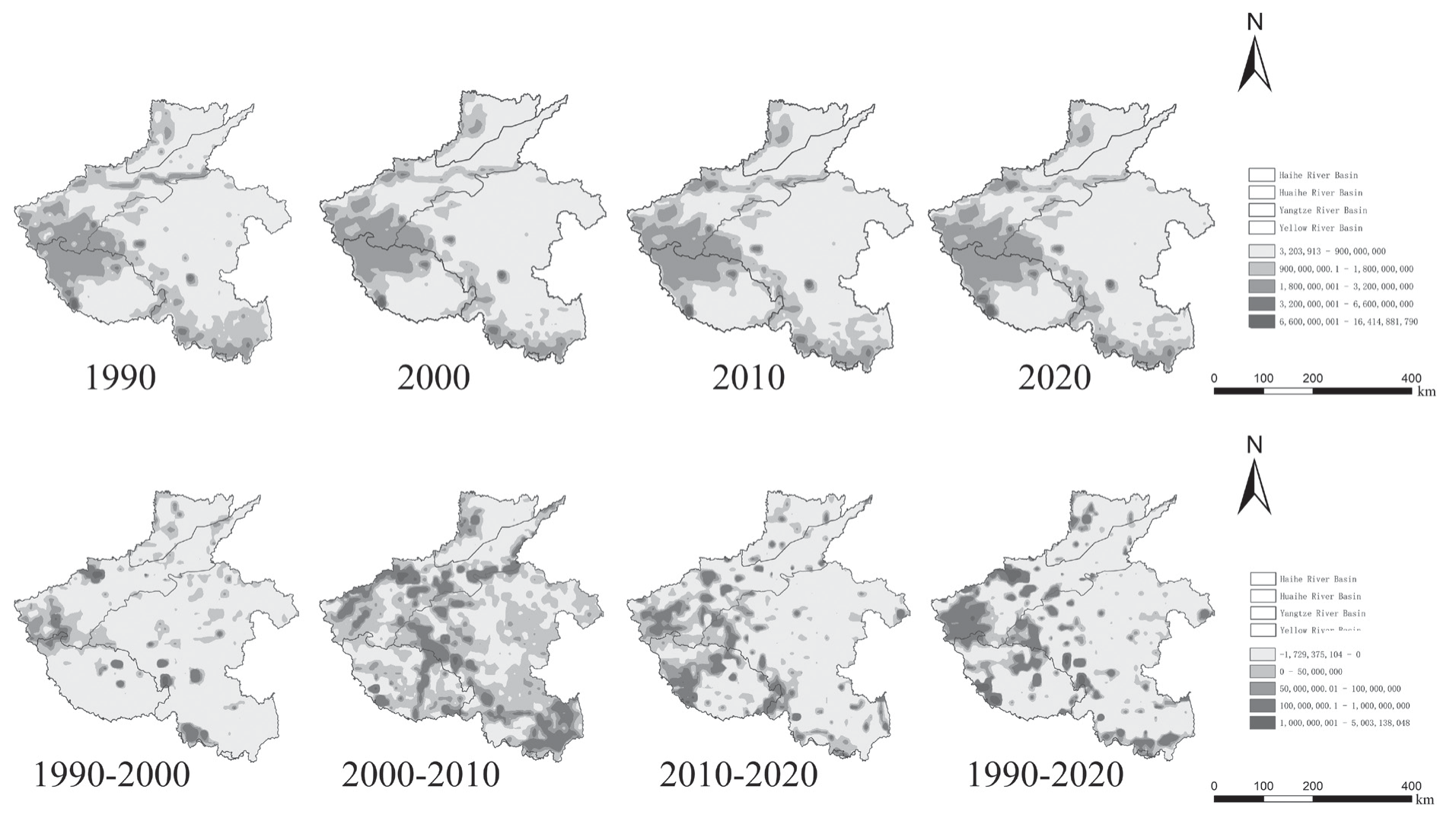
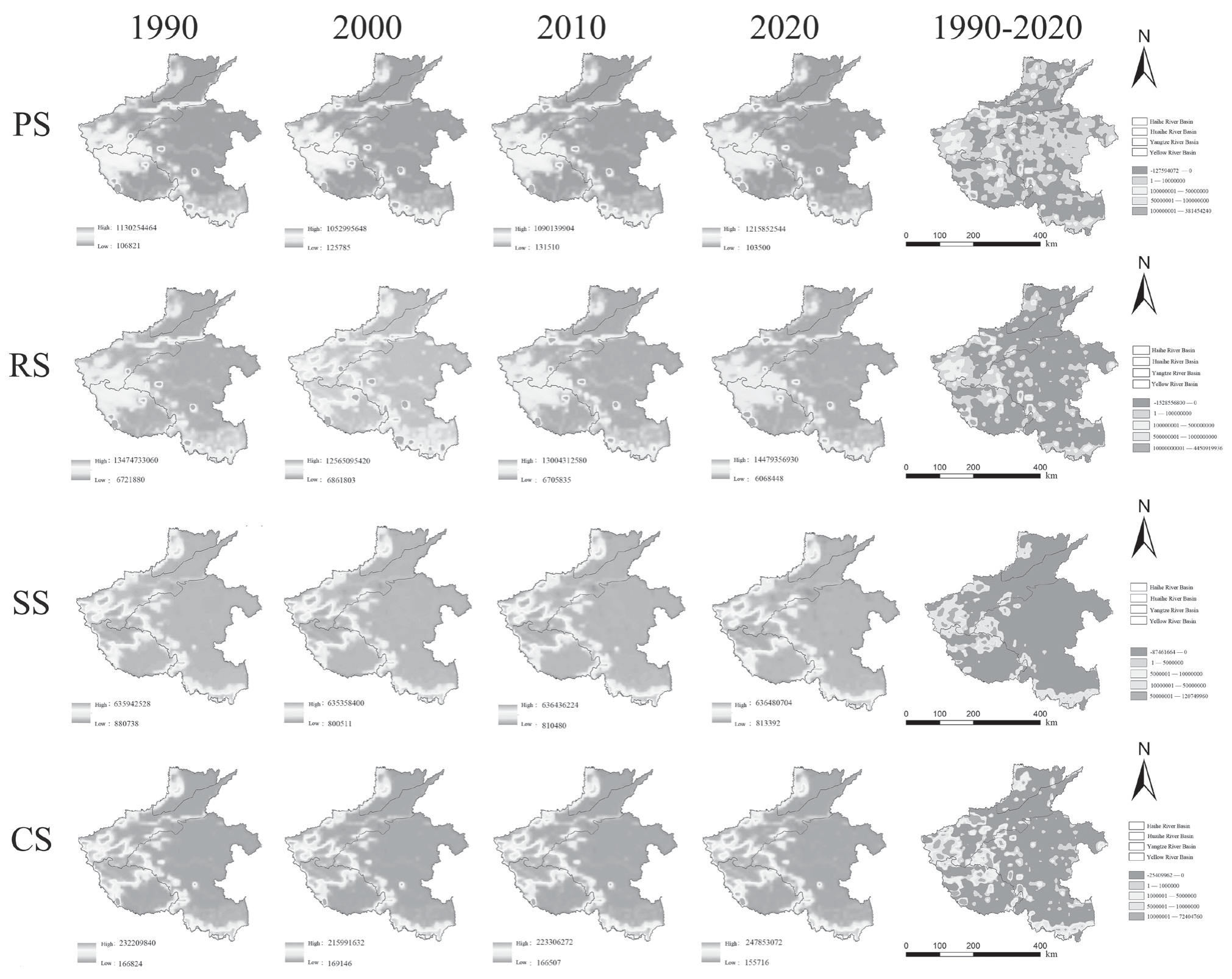
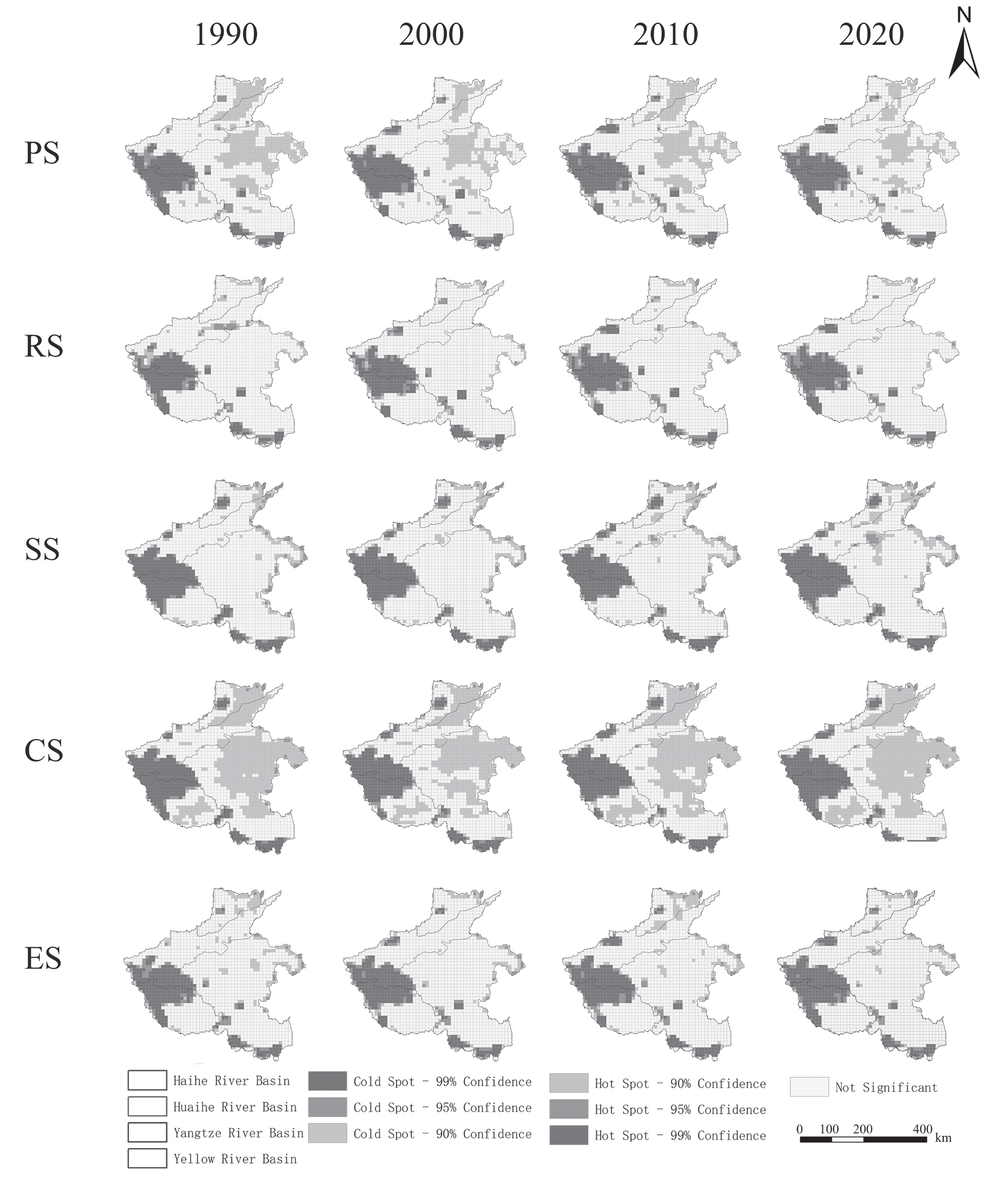
Fig. 7 shows the spatial distribution of and changes in the ESV from 1990 to 2020, with high-value areas located at the junction of YEB, YZB, HUB, and southern HUB. These areas experienced the greatest change from 2000-2010 and the least change from 1990-2000, alongside an overall yearly ESV increase. Fig. 8 shows low CS and PS values, mainly in HAB and HUB, whereas high SS and CS values occur at the YZB, YEB, and HUB junctions. Except for a notable RS change in 2000, the distribution characteristics are similar across years. The regions with decreasing RS and CS values and increasing SS and CS values are similar. PS changes are more fragmented and inconspicuous. Most regions experienced varying increases, except HUB, which decreased. The SS and CS values increased significantly, and the changes in the SS values differed from those in the RS, PS, and CS values in YZB. The SS values in YEB increased, whereas decreases occurred mainly in HUB-dominated areas.
Table 4.
Changes in ESV of different land use types in HNP from 1990 to 2020 (billion CNY).
ESV Sensitivity Test Results
Sensitivity analysis serves as a crucial approach for determining the dependence of ESV on land use. The accuracy of ESV increases when the absolute value of the sensitivity coefficient approaches zero. Table 5 shows the sensitivity coefficients of ESV and VC in the HNP from 1990-2020. The sensitivity indices for each type of land use are less than 1, suggesting the inelasticity of ESV. The grassland had the highest index, with an average value of 0.259, followed by the water. Conversely, the sensitivity indices for unused land, forests, and cropland are all less than 0.1, which substantiates the credibility of the accounting results. All the sensitivity coefficients hovered around zero, indicating a stable relationship between the ESV and the unit ESV.
ESV Trade-Off/ Synergy Evaluation
In the HNP, 55 combinations of trade-off/synergistic relationships exist among the ESs, with 9 representing trade-off relationships and 46 representing synergistic relationships. This finding indicates that synergistic relationships are prevalent among the ESVs (Fig. 9). All the trade-off relationships identified are related to SS, whereas synergistic relationships are more prominent among RS, SS, and CS. In 1990, the principal trade-off relationship was observed between FP and other services. The trade-off relationship was most significant between FP and the provision of WS (r = -0.76, P<0.01), followed by the trade-off relationships with CR (r = -0.41, P<0.01), RM (r = -0.41, P<0.01), and the rest, as mentioned above. Other notable trade-offs were primarily observed between WS and the maintenance of MN (r = -0.25, P<0.01). The pattern of trade-offs from 2000-2020 echoed that observed in 1990. Service functions predominantly exhibit synergies. There was a strong synergistic relationship between RM, SR, CR, GR, and BP. A robust positive correlation exists between RM and GR, followed by strong positive correlations between CR and SR and between CR and BP. These relationships have correlation coefficients of 1 (P<0.01), 0.99 (P<0.01), 0.99 (P<0.01), 0.99 (P<0.01), and 0.99 (P<0.01), respectively.
Spatial Autocorrelation Analysis of ESVs
This study utilized the spatial autocorrelation model to examine the spatial correlation characteristics of ESVs in the HNP spanning the period from 1990-2020. As per the spatial autocorrelation results of the ESVs presented in Table 6, the global Moran’s I values for PS, RS, SS, and CS in 1990, 2000, 2010, and 2020 were >0, with P values <0.01 and Z values >2.58, respectively. The likelihood of data clustering surpassed that of a random distribution, leading to a notable rejection of the original hypothesis. ESVs in HNP displayed pronounced spatial clustering distribution characteristics and exhibited statistically significant hot or cold spot clustering patterns in space. However, divergences in Moran’s I values and their fluctuations are observed among different ESVs. Specifically, compared with their respective ES values, the ESVs of CS recorded the highest Moran’s I values. The Moran’s I values for SS were relatively high, exhibiting a trend that initially decreased and then increased, whereas the Moran’s I values for PS and RS were lower, presenting a trend that initially increased, then decreased, and subsequently increased again.
Fig. 9.
Ecosystem service value trade-off/collaborative correlation coefficient in HNP from 1990 to 2020.
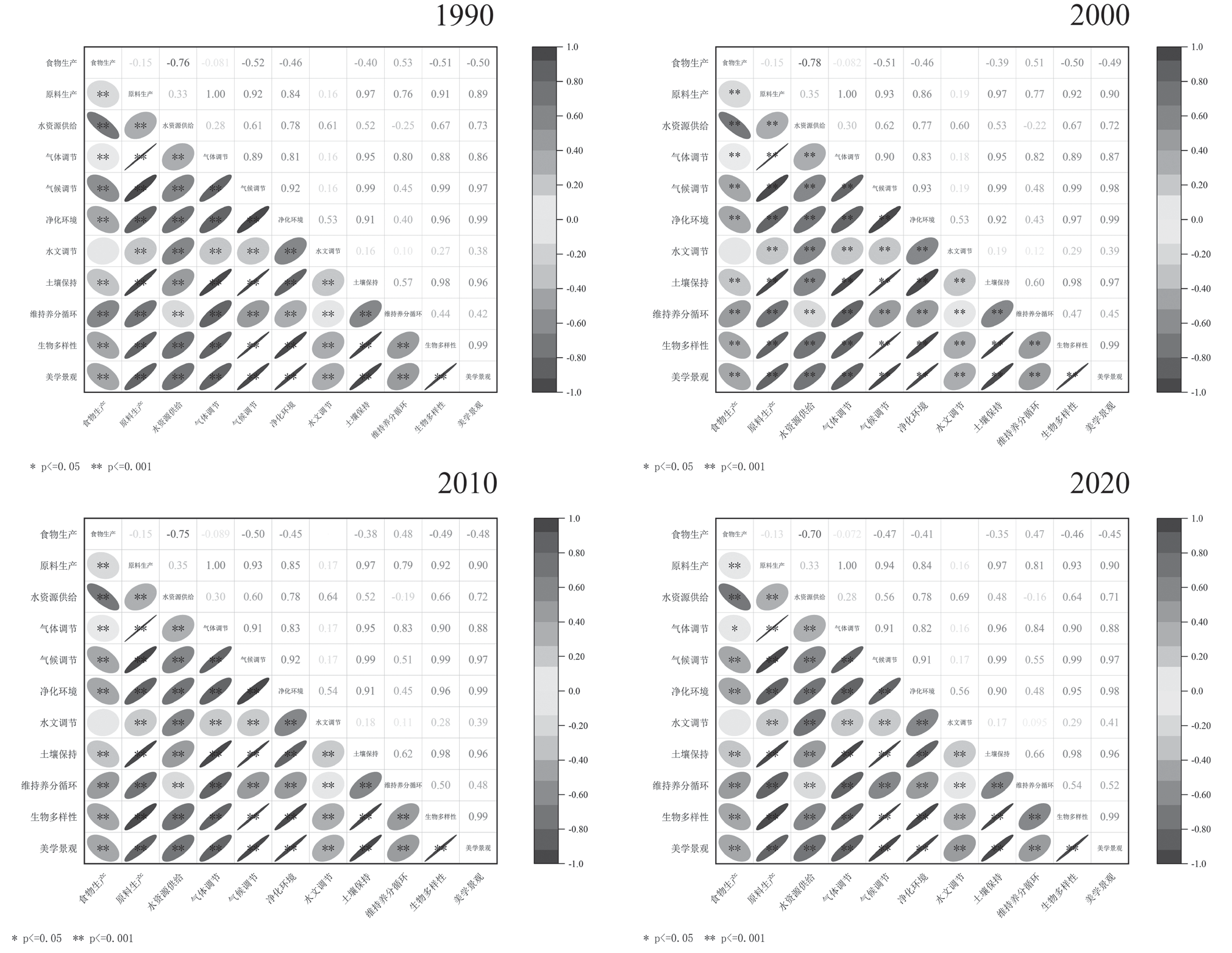
Table 6.
Global Moran’s I index variables in the study area.
The heterogeneous ESV units were identified by the Getis‒Ord Gi*. To elucidate the spatial heterogeneity of ESVs in HNP more effectively, hot spot analysis was employed to uncover the local spatial representation of ESV variation (Fig. 10). On the basis of the comprehensive analysis of ESVs in HNP, cold spots were predominantly located in the HAB and HUB, whereas hot spots were chiefly found at the junction of HUB, YEB, and YZB. Among the four distinct types of ES, PS and CS presented similar distributions and trends. Within a 0.1 confidence interval, cold spots were distributed mainly in YZB, whereas hot spots were located primarily in YEB and the southern region of the HUB. As time progressed, the demarcation of hot spots and cold spots became increasingly distinct. The cold spot area for SS expanded, the cold spot area for PS contracted, and the overall distribution of SS mirrored that of CS.
Variability Analysis of ESV Among the Four Basins
In this study, we used one-way ANOVA to analyze significant differences in the four ecosystem service types across various functional areas and years. The significant differences among ES types within diverse functional areas are designated by letters (a, b, c, d), with identical letters indicating nonsignificant differences and differing letters indicating significant differences. The vertical coordinates represent the mean ESVs in different basins. As Fig. 11 shows, ESVs from four basins – PS, RS, SS, and CS – display varying levels of significance each year.
According to Fig. 11, the PS and RS values showed notable disparities across years. The differences between YEB and YZB for PS and RS were minimal from 1990-2020. In 2000, a significant difference was observed among all four basins. Over time, differences in the PS, SS, and CS values among the basins became less significant. The RS differences among basins were significant in 1990 and 2000 but not between the YEB and YZB in 1990 and 2010 or between the HUB and HAB in 2020. ESV fluctuations and differences among basins varied by year. From 1990-2000, only the PS in HABs increased, whereas the other ESVs decreased. From 1990--2020, the PS, RS, SS, and CS values increased in the HUB, YEB, and YZB but decreased in the HAB. Overall, the PS values increased by 1.85% to 6.95% across basins, the RS values increased by -2.07% to 1.35%, the SS values increased by -0.11% to -5.39%, and the CS values increased by 0.27% to 2.71%. Basin-specific ESV differences across years were ranked as YEB>HUB>YZB>HAB, reflecting differentiated ESV development over 10-year intervals.
Correspondence Analysis between Basins and ESV
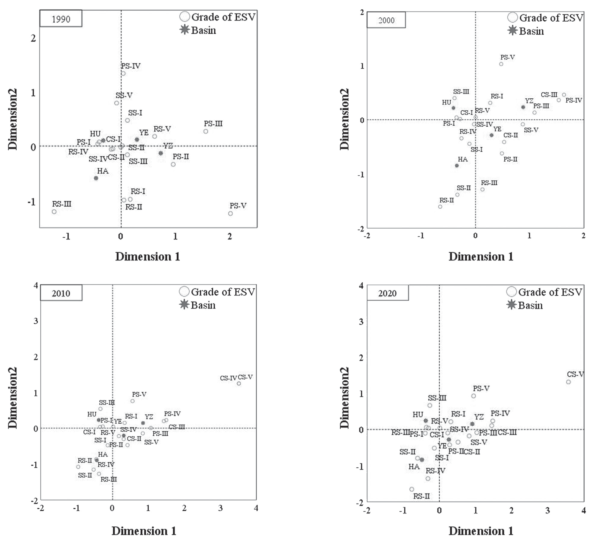
Correspondence analysis, a multivariate statistical method, was used to classify four ESVs from different basins into five categories via the equal interval method. Fig. 12 shows the correspondence between the four basins and ESVs of various ages over different years. The basins were positioned in separate quadrants, indicating significant variations in the ESV distribution. ESVs were more concentrated in 2010 and 2020 and more dispersed in 1990 and 2000. High-value areas (CS-V, RS-V, PS-V, and SS-V) were concentrated in YZB, whereas other high-value areas (CS-IV, RS-IV, PS-IV, SS-IV, RS-III, and PS-III) were concentrated mainly in YEB and HUB. Low-value areas (SS-I, RS-I, CS-I, and PS-I) were located around HABs. In 1990, YZB exhibited significant distribution characteristics and was composed mainly of ESVs such as PS-IV, SS-V, RS-V, and CS-V, whereas ESVs such as PS-I, SS-I, and CS-I were in HUB. Various ESVs were distributed mainly in HUB in 2000. From 2010-2020, high-grade ESVs such as PS-V, SS-V, RS-V, and CS-V were predominant in YZB, whereas the other ESVs were present mainly in HAB and YEB.
Discussion
Effect of Land Use Changes on ESV
Rapid urbanization and economic growth in the HNP from 1990-2020 led to notable land use transformations, impacting ESV [52]. Forest and water body ESVs initially declined but later rebounded by 513.3 billion CNY and 541.7 billion CNY, respectively, due to ecological conservation efforts and policies. Conversely, cropland, grassland, and unused land ESVs gradually decreased by 752.3 billion CNY, 305 billion CNY, and 0.2 billion CNY, respectively. Cropland decline is attributed to efficient agricultural technologies and land reconfiguration. Forests, which offer long-term ecological benefits, have expanded due to ecological management policies [53, 54]. Although water areas have expanded modestly to 2056.14 km² over three decades, they are crucial for ecological stability. Unsustainable practices such as urban sprawl, mineral extraction, and construction led to grassland degradation and ESV decline [55]. Population growth and economic development intensified unused land use, reducing ESV despite increased land area.
Fig. 11.
Differences among the values of four ES types obtained for different years and basins (lower case letters (a, b, c, d) above bars represent significant differences (P < 0.05) for the same ecosystem service type among different basins, error bars represent 95 % confidence intervals).
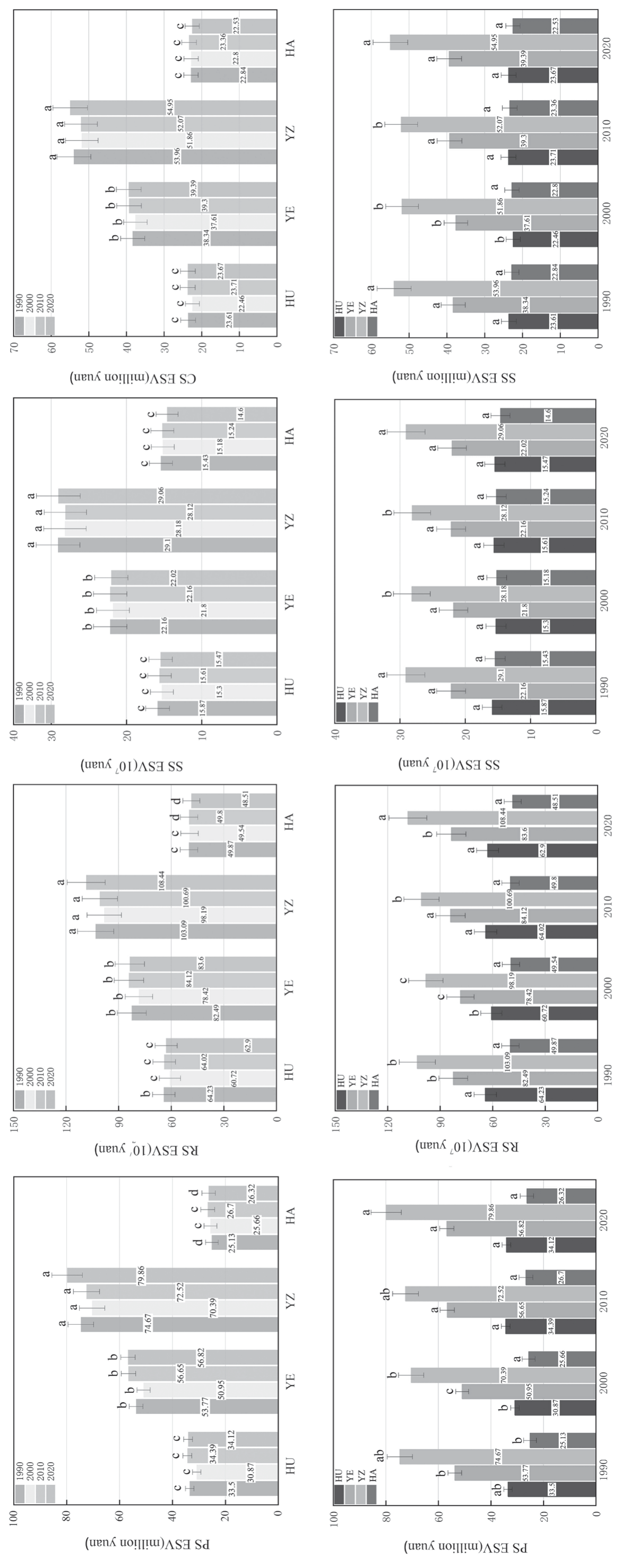
Fig. 12.
Corresponding analysis of each watershed and ESV from 1990 to 2020 (the four graphs represent the corresponding relationship between the three basins and ESVs from 1990 to 2020).
Spatiotemporal Variation Characteristics of ESVs in the Four Basins and the Trade-Offs/ Synergies of ESS
The ESV in HNP varies spatially, with YZB and YEB having notably higher ESVs than HUB and other regions due to distinct LULC patterns. At the confluence of YZB, HUB, and YEB, forests, grasslands, and unused land with abundant vegetation contribute to higher ESVs, whereas plains with sparse vegetation in HUB’s east and parts of YZB favor agriculture and urbanization. Both human and natural factors influence ESV trends. Since 2000, ecological restoration has improved soil, water, and vegetation. Policies such as ecological redlining and land-use changes reflect preservation efforts. ESV hot spots are correlated with high LULC diversity, especially at confluences, whereas cold spots are located at peripheries. Over three decades, increasing ESV hotspot aggregation has suggested an increase in high ESV areas and a decrease in low ESV areas due to evolving LULC patterns [56]. In HNP, ESs have complex trade-offs and synergies, with synergies prevailing. Trade-offs, such as RM and CR, occur mainly between the FP and other services because of conflicts between agriculture and ecological protection. Spatial heterogeneity affects the trade-off between FP and SR. Synergistic relationships exist between AL values and BP and among RM, CR, and SR, highlighting the positive contributions of grasslands and forests to climate, biodiversity, and soil [57, 58]. Considering this, ESV synergies are crucial for enhancing ecological functions.
Differences in the ESVs in Different Basins
A comprehensive spatial analysis of regional elements is essential for effective ecosystem management [59]. Understanding ecosystem composition, structure, and functional attributes, as well as developing context-specific strategies, is crucial for sustainable restoration or preservation. Recent land use fluctuations in HNP basins have led to significant ESV variance, necessitating diverse ecological management strategies to harness the leadership roles of ecosystems and promote sustainable progress.
YZB, with a superior ecological environment and moderate economic development, requires the identification and optimization of its ecological security framework while sustaining growth. This can be achieved through ecological restoration projects, sustainable land-use practices, and policy interventions. HAB, although ecologically endowed, lags in economic development and needs protection from anthropogenic harm, along with interbasin ecological protection mechanisms for sustainable resource management. HUB, benefiting from its strategic location, has undergone comprehensive development, but progress has exacerbated ecological land degradation and reduced ESV. Future strategies must balance economic growth and ecological preservation, upholding the “returning farmland to forests” policy to expand green vegetation and mitigate the impacts of urbanization and industrialization. YEB requires ecological restoration and reduced environmental impact, prioritizing optimized land use, delineating urban development boundaries, and promoting sustainable practices.
ESV disparities among basins highlight the need for tailored ecosystem protection and management measures [60]. A comparative analysis of ESVs revealed a general increase in the PS values from 1990-2020, whereas the SS values decreased, particularly in the plains areas, due to rapid urbanization and economic expansion. National policies prioritize ecological environment protection, coinciding with increases in PS, RS, SS, and CS values across all basins from 2000- 2020. Distinctive annual ESV distribution patterns are identified, notably in HUB with lower-level ES values. YZB, with Asia’s longest river and fragile ecological environment, requires focused efforts to establish vegetation, prevent soil erosion, and maintain ecosystem stability. By 2000, intermediate ESV levels were predominant in HAB and YEB, evolving to advanced ES functions by 2010, particularly in YEB. From 2010-2020, YZB exhibited high-quality ESV, underscoring its ecological richness. Comprehensive ecological protection and systematic restoration efforts are paramount in the HUB to optimize land use arrangements across the region.
Recommendations for Ecosystem Management in Different Basins
Recent studies have revealed significant land use patterns and ESV shifts across various basins within the HNP, necessitating tailored ecological management strategies. The aim is to foster sustainable ecosystem progression and stewardship. Regional planning must align with dominant ecosystem types, features, and importance. The disparities in ESVs highlight the need for targeted protection and management.
YZB, with its exceptional ecology and economic development, requires enhancing its ecological security while maintaining progress. HAB, despite its ecology, lags economically, necessitating protection from anthropogenic harm and interbasin conservation mechanisms. HUB development has intensified land degradation and reduced ESV, promoting a balance between growth and preservation through “returning farmland to forests” and increasing green coverage. For YEB, ecological restoration and impact minimization are crucial, with a focus on optimizing land use to reduce the ecological footprint.
Defining urban boundaries and avoiding ecosystem conversion are essential. Reinforcing urban green spaces alleviates environmental pressures. Tailored ecological conservation strategies, which are founded on precise ESV estimation, are vital. Establishing protection standards suited to each basin’s characteristics and fostering stakeholder involvement are also important. The exploitation of vital resources safeguards ecological integrity. Optimizing land use to protect local ecosystems promotes sustainability and resilience. Delineating ecological protection red lines enforces control over critical spaces. Setting differential standards, prioritized as HUB>YEB>HAB >YZB, ensures efficient, tailored interventions. These should include mandatory and incentivized measures for protection and restoration, facilitating effective management and nurturing sustainable development across HNP diverse landscapes [61].
Limitations and Prospects
This study employed the value equivalence method to calculate tailored ESVs for HNP, considering various land use types and distinguishing PS, RS, SS, and CS. The evaluation models for 11 secondary ES provided a comprehensive assessment. However, ESV computation lacks a universal standard, leading to neglect or lack of measurement of some aspects. Future research should integrate statistical methodologies with model simulations to evaluate long-term policy impacts on ESs. Scenario simulations that consider environmental protection, economic development, and natural dynamics are crucial for assessing future ES changes and tradeoffs/synergies. Expanding datasets to explore the driving mechanisms behind ESV evolution is essential for enhancing regional ecological protection, contributing to a more comprehensive understanding and effective management and ultimately promoting sustainable development and ecological resilience in HNP.
Conclusions
This study conducted a detailed evaluation of land use changes in HNP basins via the land use transfer matrix and quantified ESVs via the equivalent factor method. The findings, validated through sensitivity analyses, highlighted the importance of incorporating land use dynamics into ecological planning. Construction land showed the most significant increase, whereas grassland and cropland areas decreased, indicating urbanization pressures. Forests and aquatic regions initially declined but later recovered, emphasizing the need for their conservation. The spatial distributions of the land use categories varied across the four basins, with distinct trends in the ESVs. HUB had the highest cumulative ESV, followed by YEB, YZB, and HAB. Synergistic relationships among ESVs, particularly between RS and SS and between CS and PS, were observed, highlighting the interconnected nature of ecosystem services. Tradeoffs were associated mainly with PS, necessitating careful land use planning and resource allocation. The spatial distribution of ESVs exhibited correlation and aggregation patterns, with cold and hot spots concentrated in specific basins. The variations in ESVs across different basins and timeframes emphasize the importance of considering the local context and basin-specific characteristics in management strategies. This study provides insights into the interplay of ESVs across HNP basins and emphasizes the need for integrated approaches that balance human activities with ecological preservation to ensure long-term sustainability. These findings serve as a model for similar regions and contribute to a broader understanding of land use and ESV dynamics within the framework of sustainable ecological management.