

Introduction
Iron ore tailings are the main waste product from iron ore mining, and these waste materials are often stored in the open air. Many studies have demonstrated that this crude storage method leads to the spread of harmful substances in the tailings into the atmosphere, soil, surface water, groundwater, and other environments through external forces such as wind and rain, and produces erosive pollution in the surrounding environment [1-4]. Heavy metals are elements with an atomic density greater than 5.0 g/cm3, such as Cr, Cu, Cd, Pb, Hg and Zn [5, 6]. Among them, chromium is one of the three heavy metal elements recognized by the international community as carcinogenic, and at the same time, chromium is very difficult to migrate from the soil, thus making chromium one of the priority pollutants for soil monitoring.
After years of stockpiling, heavy metals in tailings are spread by water and wind erosion, thus directly threatening the surrounding water and soil environment. Additionally, these heavy metals accumulate in animals, plants, and humans [7, 8], meaning that the heavy metal contents in tailings and surrounding soils pose a direct threat to human and environmental health [9].
Therefore, there is a pressing need to develop novel methods to quickly and accurately estimate heavy metal chromium contents in tailing ponds and surrounding soils. In turn, this would enable the establishment of more effective ecological protection and mine management strategies. Conventional methods for the quantification of soil heavy metal chromium content via field sampling and laboratory analysis are highly accurate. However, these methods are time-consuming and labor-intensive and are not well suited for the monitoring and assessment of soil heavy metal chromium pollution in large areas, which limits their wide applicability [10]. In contrast, the rapid development of hyperspectral technology provides a new way to conduct quantitative analysis of chromium based on the non-destructive, dynamic, macroscopic, and efficient acquisition of surface information [11]. Hyperspectral can obtain rich spectral information, which can enhance the spectral response characteristics. In addition, the continuous improvement of band selection algorithms and the application of different modeling methods are reported in many research results on soil heavy metal estimation. For example, in a study of arsenic concentration in the soil of an open-pit coal mine, a three-band spectral index was constructed by combining the spectral information and soil clay minerals, which led to the enhancement of arsenic estimation accuracy with the highest correlation coefficient and the lowest RMSE (r = 0.9732, RMSE = 0.0703) [12]. In another study, it was proposed that algorithms such as wavelet transform and random forest can effectively improve the inversion accuracy [13, 14], and all of these results show the applicability of hyperspectral technology in the evaluation of soil heavy metal pollution [15, 16]. However, the sources and distribution of heavy metals in tailing areas are very complex [17].
This study analyzed the Sijiaying iron tailings reservoir in Luanzhou City, Hebei Province, and the spectral information of the soil was collected in the laboratory based on field sampling. Moreover, the amount of chromium in the soil samples was determined using inductively coupled plasma-mass spectrometry (ICP-MS). The inverse model of soil chromium content was established by using the partial least squares regression and multiple linear regression methods, and the accuracy of these approaches was verified and analyzed to confirm whether they could be applied for the rapid monitoring of soil heavy metal pollution in high-silica Anshan-type iron tailings.
Experimental
Sample Data
This study analyzed soil samples from the Sijiaying iron tailings pond and the surrounding area in Luanshi City, which is an Anshan-type sedimentary metamorphic iron ore deposit [18]. According to the geographical distribution characteristics of the tailing ponds in the study area, the sample points were taken approximately 10-20 cm below the surface layer. In a unit area, soil samples were collected according to the east, west, south, north, and central points, and then these 5 soil samples were mixed into 1 combined sample to obtain a total of 43 combined samples. The soil samples collected in the field were cleaned of roots, branches, leaves, stones, etc., and then put into glassware and dried in a dry and ventilated environment. After 24 h drying, each sample was weighed at 500 g, put into a triturator for grinding, and then filtered through a sieve with a diameter of 0.15 mm after grinding. Each soil sample is divided into two parts: one part is used to determine the chromium content, and the other part is used for spectral measurement.
The 4 mg sample was weighed by an analytical balance and placed in a polytetrafluoroethylene digestion tube. 3 mL nitric acid, 3 mL hydrochloric acid, and 0.5 mL hydrofluoric acid were dripped into the sample digestion tube and heated for digestion by an electric heating plate. After digestion, the digestion tube was naturally cooled to room temperature, and the digested samples were filtered and diluted with deionized water into a 10 mL volumetric bottle and mixed evenly. The heavy metal chromium content was determined by an inductively coupled plasma mass spectrometer (ICP-MS), in which each sample was measured twice in parallel, and the average value was selected as the final content.
Spectrum Collection and Measurement
Spectral profiles of soil samples were collected using an ASD hyperspectrometer at a spectral range of 350-2500 nm. Spectral data were obtained in a dark room by placing the soil samples in a 10 cm * 10 cm * 2 cm black box and placing them flat on a horizontal table with a black cloth background. Measurements were made with the probe touching the soil sample, and each sample was measured five times. The actual reflectance spectral curve for each sample was plotted using the average of the measured spectral curves. The inverse transformation of the spectral reflectance enhances the spectral differences in the visible region. Moreover, to eliminate baseline drift and background interference effects and improve the spectral resolution, the inverse transformed spectra were preprocessed using the second-order Savitzky-Golay (S-G) derivative method with a window of 5 [19].
Spectral Feature Preference
Based on the analysis of the response characteristics of soil reflectance to heavy metal content, the characteristic bands were selected using three methods: successive projections algorithm (SPA), competitive adaptive reweighted sampling (CARS), and correlation analysis. Sensitive bands are often determined by correlation analysis between soil heavy metal content and spectral reflectance, the higher the correlation, the more sensitive the band is. Accordingly, the sensitive band reflectance extracted from the correlation analysis and the soil heavy metal chromium content are subjected to stepwise and partial least squares regression analyses, and the inverse model for the heavy metal chromium content in the soil is established. The correlation is usually denoted by a letter and is used to measure the linear relationship between two variables [20].
Table 1.
Comparison of different band selection methods.
where Cov(X,Y) is the covariance of X and Y, Var[X] is the variance of X, and Var[Y] is the variance of Y.
Results and Discussion
This study uses multiple linear regression (MLR) or partial least squares regression (PLSR) to model the data obtained after processing using three characteristic band selection algorithms, after which their prediction accuracy was compared. The full spectrum has 1075 bands and the correlation analysis extraction 70 band points. The characteristic band selection of the spectral data is performed using the CARS algorithm with 100 Monte Carlo (MC) sampling times and 8 characteristic bands. The feature bands were selected using the SPA method, at which time the number of feature bands was selected to be 18. The MLR model was constructed for the 18 feature band points extracted by SPA and the 8 feature band points extracted by CARS, and the RC correction, prediction correlation coefficient (RMSEC), RP correction, root mean square error of prediction (RMSEP), and RPD values of the model are shown in Table 1. Upon comparing the prediction performances of the three feature band selection algorithms, our findings indicated that SPA selects only 18 feature band points with an RMSEP of 6.2 and an RPD of 2.5, and therefore this approach was considered to have the best prediction performance. SPA not only reduces the complexity of modeling but also greatly improves the prediction accuracy of the model [21].
Fig. 1.
Shows the effects of the inversion of different models. a) FULL-PLS inversion effect, b) SPA-MLR inversion effect, c) CARS-MLR inversion effect, d) CA-PLS inversion effect.
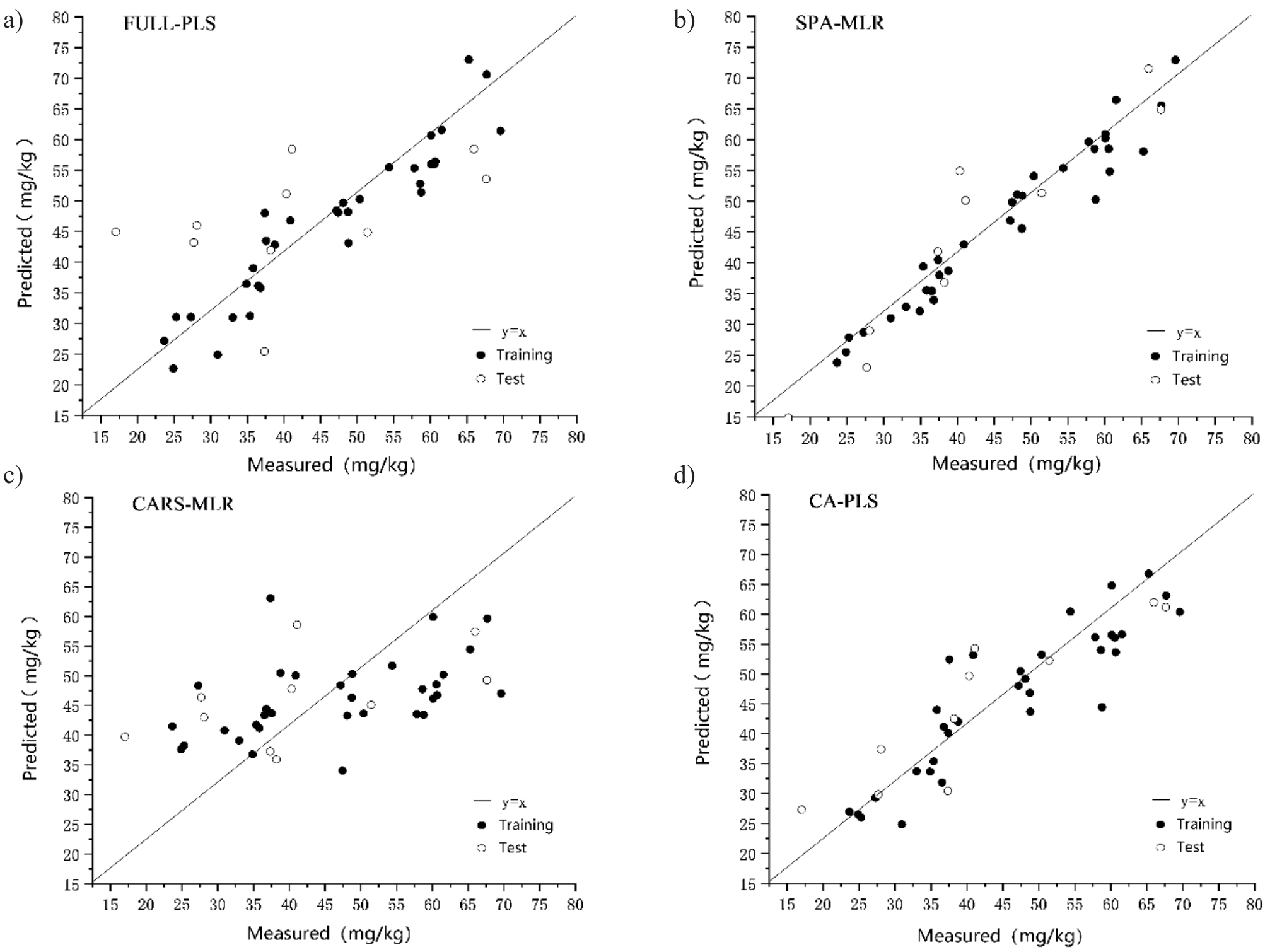
Fig. 1 shows the correlation plots between the measured and predicted values of soil chromium content for different models for the prediction sample sets. The oblique line in the figure is the trend line y = x, and the model fitting effect is mainly reflected by the distance between the scatter point and the trend line. The closer the distance, the higher the precision. As can be seen from Fig. 1b), only a small number of samples are far from the trend line, and most of the dispersion points are close to the trend line. Therefore, the SPA-MLR model of the chromium element has the best fitting effect.
Conclusions
This study measured the soil spectral information of the Tangshan iron tailing area by hyperspectral technology, and inverse modeling of soil chromium content in the tailing area was conducted using three characteristic waveband extraction methods combined with multiple linear regression and partial least squares regression. The following are the main conclusions of this study:
(1) The model established using the SPA-MLR method coupled with hyperspectroscopy was superior to the other models and could thus be used to accurately estimate the chromium content in soil samples collected from the Tangshan iron tailing area.
(2) The model constructed based on the SPA-MLR method exhibited an RC of 0.9, an RMSEC of 4.7, an RP of 0.9, an RMSEP of 6.2, and an RPD value of 2.5, which is better than the other models in terms of prediction accuracy.
(3) The number of samples directly determines the model accuracy. Our experiment only contained 43 samples, which cannot effectively express the relationship between the number of samples and the model estimation accuracy. Therefore, future studies will assess the degree of influence of the number of samples on model accuracy and root mean square error.

