

Introduction
Macroalgae blooms (MABs) have increased remarkably in the global oceans in recent years, becoming a worldwide marine ecological problem [1-3]. Since 2007, MABs caused by outbreaks of Ulva prolifera have been occurring periodically in the Yellow Sea. The MAB in the Yellow Sea (“green tide”) is generally considered to be the world’s largest transregional MAB because of its long duration, wide influence area, and the great difficulty associated with cleaning it up [4]. It has become the most serious marine ecological disaster in the Yellow Sea, causing serious ecological, environmental, and socioeconomic problems and threatening the sustainable development of the ocean [5]. Many studies have shown a strong interest in identifying the origin and causes of MAB outbreaks [4, 6, 7], clarifying the development process [8, 9], and addressing their environmental impacts [10-14]. Satellite data plays a crucial role because of the advantages of multi-scale, multi-spatial resolution, and large-area repeated observations in many studies. With the help of satellite data, the patterns associated with green tides are well understood, especially their origin, development, and drift mechanism [8, 15-18].
Optical images, such as GOCI (Geostationary Ocean Color Imager), MODIS (Moderate Resolution Imaging Spectroradiometer), HJ-1A/1B (HuanjingJianzai- 1A/1B), GF-1 (GaoFen-1), and HY-1C (Haiyang-1), are widely used in monitoring MABs [5, 17, 19-22]. However, the MAB in the Yellow Sea is the result of a dynamic process. Few remote sensing sensors have both fine spatial resolution and high temporal resolution. In addition, during the MAB outbreaks (occurring in early June to early August), it is the rainy season in the Yellow Sea due to the influence of the East Asian summer monsoon. This results in images that are often obscured by cloud and fog [23]. The combining of multi-source data can increase the number of available images and combine the advantages of fine spatial resolution images (i.e., GF-1 and Sentinel-2) and high temporal resolution images (i.e., GOCI and MODIS). However, the size of macroalgae patches varies from several centimeters to several kilometers [24]. Thus, the spatial resolution difference of multi-source data has a significant impact on the detection of macroalgae [25]. For example, the relatively coarse resolution (250 m) of MODIS is likely to miss the small patches [26], while GF-1 is better for detecting small macroalgae patches with finer resolution (16 m) [27]. As a result, the coverage area estimated by multi-source data varies significantly because of pixel-mixing. The error between the coverage area estimated by coarse resolution images and by fine resolution images can be as high as 60% or even 200%. The larger the difference in spatial resolution, the larger the error [28]. The pixel un-mixing method and the relational model method can effectively reduce this error, but there is still an error of about 30%, restricting the precise formulation of MABs prevention and control strategies [15, 29- 32]. If there were a satellite with both high temporal resolution and fine spatial resolution, there would be no error problem. HuanjingJianzai-2A/2B (HJ-2) is just such a satellite.
The HJ-2 series satellites are part of the Chinese Environmental Protection and Disaster Monitoring Satellite Constellation developed by China. The first two (HJ-2A and HJ-2B) series satellites were launched from the Taiyuan Satellite Launch Center of China on 27 September 2020 to replace the HJ-1 that had been in orbit for 12 years. Each satellite is equipped with four imaging sensors, including a wide-view charge-coupled device (CCD) camera, a hyper-spectral imager (HSI), an infrared multispectral scanner (IRMSS), and a polarized scanning atmospheric corrector (PSAC). The CCD camera, HSI, and IRMSS are used primarily for surface observations, and PSAC is used mainly to monitor atmospheric components such as water vapor and aerosols [33]. Compared to HJ-1, the data acquisition ability, technical performance, and data accuracy of HJ-2 have been greatly improved. The revisit period of both satellites’ CCD cameras is only 2 days after networking. Moreover, the CCD cameras have a fine spatial resolution (16 m), and they can operate with GF-1 and GF-6 satellites equipped with a wide field of view (WFV). Thus, 16-m resolution images can achieve global coverage in 1 day. In this work, the MABs monitoring results of HJ-2 CCD images and GF-1 WFV images were compared to analyze the macroalgae detection ability of HJ-2. HJ-2 CCD images of different time phases were acquired to dynamically monitor the MABs distribution in the Yellow Sea in 2022 and research the application performance of HJ-2 in monitoring MABs.
Materials and Methods
Study Area
The Yellow Sea (31°40′N–39°50′N, 119°10′E–126°50′E) is a marginal sea of the western Pacific Ocean, lying between mainland China to the west and north and the Korean Peninsula to the east, and linking the Bohai Sea in the northwest with the East China Sea in the south. The Yellow Sea is usually separated into the North Yellow Sea and the South Yellow Sea by a line running from Chengshantou on the Shandong Peninsula to Changshan. The South Yellow Sea is where most green tides have broken out in recent years [15, 21]. The study area is within the range of 32°N–38°N, 119°E–123°E in the South Yellow Sea (Fig. 1), where MABs have occurred for 17 years since 2007.
Remote Sensing Data and Processing
The HJ-2 satellite data used in this work were obtained by the CCD sensor with 16 m spatial resolution, including the five bands of blue, green, red, red edge, and near infrared (NIR). The GF-1 satellite data used were obtained by the WFV sensor with 16 m spatial resolution, including four bands of blue, green, red, and NIR. The spatial resolution, width, and revisit period of these two satellites are consistent, and the blue, green, red, and NIR band ranges are the same. The specific parameters are shown in Table 1.
The HJ-2 and GF-1 data used in this work were Level-1 product data, which are shown as digital number (DN) values. All images were converted into TOA radiance by radiometric calibration (Eq. (1)) to avoid the influence caused by different sensors. They were transformed into the WGS_1984_UTM_Zone_51N coordinate system.
Fig. 1.
Map of the study area. The true-color image is a composite of the China & Brazil Earth Resource Satellite (CBERS)-04 wide field imager’s (WFI) band 4 (red), band 3 (green), and band 2 (blue), acquired on 25 June, 2022. The green regions show the spatial distribution of Ulva. prolifera macroalgae bloom, and the red regions show the current area affected by macroalgae.
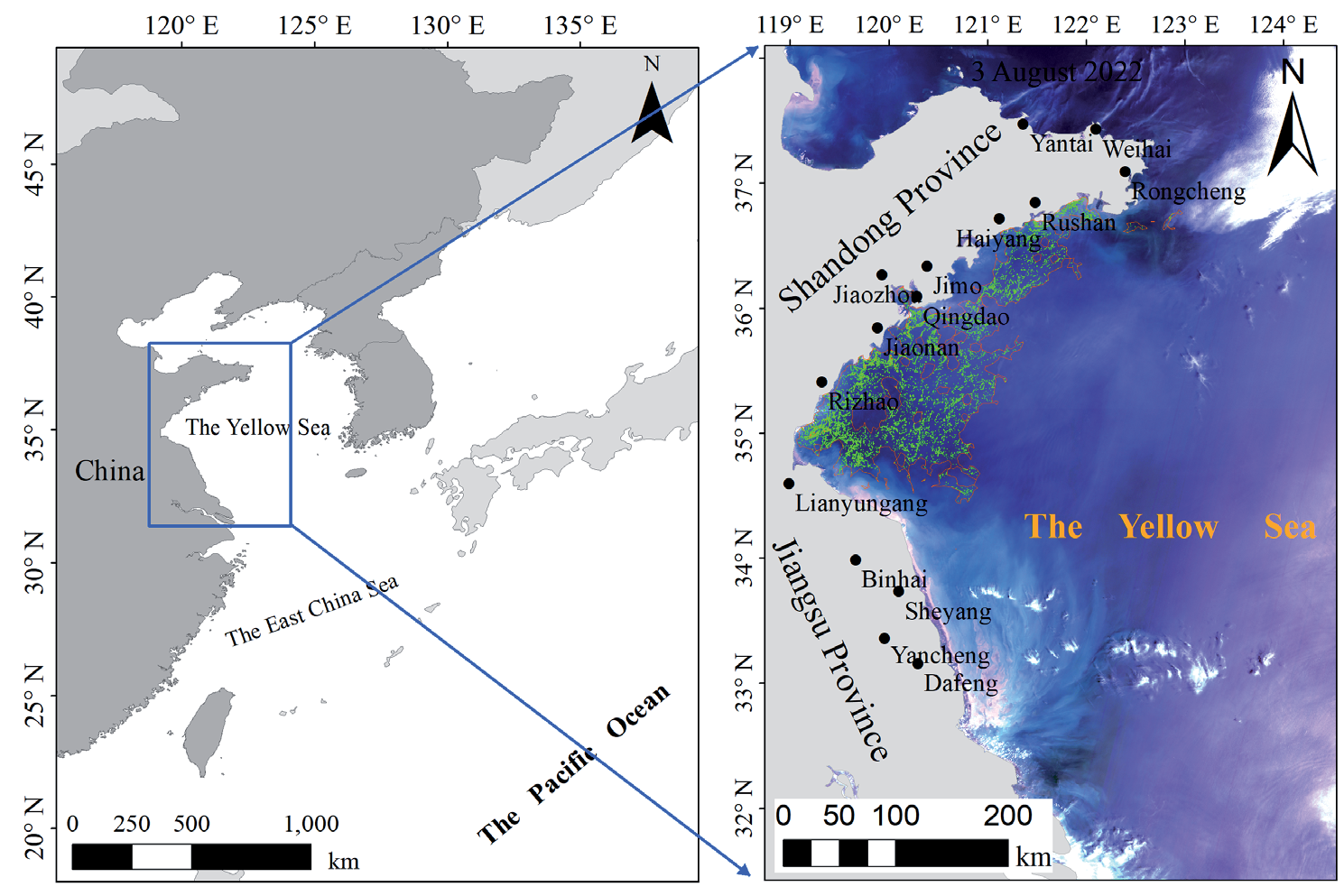
Table 1.
Parameters of the HJ-2 CCD and GF-1 WFV.
where L(λ) is the TOA radiance (w•m−2 •sr−1•μm−1) and Gain and Bais are the gain and offset values, respectively, which can be obtained from the Header File. The Fast Line-of-sight Atmospheric Analysis of Spectral Hypercubes (FLAASH) atmospheric correction module, implemented via ENVI5.6 software (Exelis Visual Information Solutions, Inc., Boulder, CO, USA), was applied to process HJ-2 and GF-1 images to derive the reflectance values (R, unitless). Subsequently, all images were transformed into the WGS_1984_UTM_ Zone_51N coordinate system after projection.
Macroalgae Detection Method and MABs Area Statistics
Many macroalgae detection algorithms have been proposed based on the distinct spectral difference between natural seawater and macroalgae-covered seawater in the red and NIR bands. Among them, difference index algorithms, such as the Floating Algae Index (FAI), Difference Vegetation Index (DVI), and Virtual-Baseline Floating Macroalgae Height (VB-FAH), are relatively unaffected by sunlight and aerosol changes [26, 31, 34]. Because HJ-2 lacks a short-wave infrared band and the detection effects of DVI and VB-FAH were similar [24], the DVI index (Eq. (2)) was selected for detecting pixels containing macroalgae in this study. This index has been widely used and demonstrated high accuracy for macroalgae detection in numerous studies [22, 24, 35].
where RNIR and RRed are the reflectance at the NIR band and red band, respectively.
Given the significant variability in atmospheric turbidity, ocean background, and sun glint, a dynamic threshold of DVI was used to detect the macroalgae [20-22, 26]. DVI images were segmented into small windows, each measuring 100×100 pixels. A set of thresholds (dependent on the optical conditions of the water surface) was used to classify, on a window-by-window basis, which pixels contained macroalgae. Pixels with DVI values exceeding the applicable threshold were considered to contain macroalgae [20, 26]. In this study, these thresholds ranged from -0.02 to 0.02. The daily coverage area of MABs (CA, km2) was derived by multiplying the pixel size of the satellite image (PS, km2) by the total number of pixels (N) that were identified as macroalgae [30], as shown in Eq. (3).
Analysis Method for Macroalgae Detection Capability of HJ-2 Satellite Images
GF-1 imagery has been widely used in MAB monitoring and comparison analysis of coarse resolution macroalgae detection capability [31, 36]. We used a GF-1 image as a reference to evaluate HJ-2’s macroalgae detection capability through three indicators.
The first indicator was the average gradient of the DVI image (G̅ , defined by Eq. (4)), which reflects the image’s ability to express small, detailed changes. It can not only evaluate the image clarity but also reflect the contrast of small details and texture changes. The greater the average gradient is, the better the image clarity and detail expression are [37-38]. G̅ was compared using image pairs selected over the same macroalgae region with the same acquisition date.
where M and N are the numbers of rows and columns of the image, respectively, and Z (i, j) is the DVI value of row i and column j.
The second indicator was the macroalgae visibility on the DVI image (V, defined by Eq. (5)), consisting of the mean DVI value difference between a pixel containing macroalgae and the background (i.e., seawater). The larger the difference, the greater the macroalgae visibility, which is more conducive to macroalgae detection. V was compared with the same image pairs as G̅ .
where Meanmacroalge and Meanbackground represent the average value of macroalgae and the seawater background on the DVI image, respectively.
The third indicator was the mean relative difference (MRD, defined by Eq. (6)) between the macroalgae patch area detected in the GF-1 image and the HJ-2 image. The smaller the MRD, the more consistent the macroalgae detecting capability of these two images. MRD was calculated using pairs of macroalgae with the same or similar distribution selected on the same acquisition date.
where N is the number of image pairs.
Four satellite images (listed in Table 2) were used to analyze the above three indicators, within a time interval of 90 minutes.
Analysis of the MABs’ Spatiotemporal Variation in 2022
HJ-2 images from 2022 with fewer clouds were selected to monitor MABs, with a total of 12 periods. The macroalgae were extracted using the method described in Materials and Methods Section and analyzed to determine their spatiotemporal variation while considering three characteristics.
The first characteristic was the variation in macroalgae daily coverage area (CA, detailed in Materials and Methods Section). The second characteristic was the variation of the area affected by MABs (AA). The AA acquisition method was to use the Aggregate Polygons Tool in ArcGIS software to aggregate macroalgae patches within a certain range and generate the polygons enveloping macroalgae patches. This polygon area was designated AA (Fig. 1). The third characteristic was the degree to which MABs were affecting the Yellow Sea, which was represented by the annual distribution density (ADD). ADD was obtained in two steps: (1) the distribution density of macroalgae (Dm) was calculated based on Eq. (7); (2) ADD was obtained by calculating the average D of all images based on Eq. (8). The larger the ADD value, the more serious the effect [21]. ADD values were divided into five equal intervals designated as L1 to L5 (low to high) based on their annual range [21].
Table 2.
Acquisition time of semi-synchronous satellite images.
| Satellite and Sensor | Acquisition time (hh:mm dd/mm/yyyy) |
|---|---|
| HJ-2 | 11:31 11 June 2022 |
| GF-1 | 10:06 11 June 2022 |
| HJ-2 | 11:35 18 July 2022 |
| GF-1 | 10:10 18 July 2022 |
where m is the mth window; Am and As are the macroalgae coverage area and the total area of the region in the mth window, respectively. The window size was 4 km × 4 km, which is consistent with our previous study [21]. Ns is the number of windows in an image, and Nimage is the number of selected remote sensing images.
Results
Comparison of Macroalgae Detection Capability between HJ-2 CCD and GF-1 WFV
Fig. 2 shows that the HJ-2 CCD images and GF- 1WFV images from two semi-synchronous periods in the same region on 11 June 2022 and 18 July 2022 were enhanced by a linear 2% stretch. From the perspective of visual interpretation, the macroalgae information on HJ-2 images is more obvious, and the visual interpretation effect of HJ-2 is slightly better than that of GF-1.
To objectively evaluate the macroalgae detection capability of HJ-2 satellite images, 10 pairs of sub-images were selected from each of these two groups of semi-synchronous images according to differences in water turbidity. Two pairs were located near the coast of Jiangsu Province, where the water is turbid, as shown in T1 and T2 in Fig. 2a) and c), and three pairs were located in the middle of the Yellow Sea, where the water is clear, as shown in Y1, Y2, and Y3 in Fig. 2a) and c). Five pairs were located near the coast of Shandong Province, where the water is relatively clear, as shown in S1-S5 in Fig. 2b) and d). In these 10 pairs of sub-images, there were some regions with a greater clustering of macroalgae, in which the macroalgae were mostly distributed in strips and patches (Y1, Y2, Y3, S1, S2, and S3). There were also several regions with less macroalgae clustering; in these regions, the macroalgae mostly exhibited a scattered distribution (T1, T2, S4, and S5). The average gradient and macroalgae visibility of these sub-images of the DVI images were counted based on the methods described in Materials and Methods Section. The results showed that the average gradient of the HJ-2 DVI images was close to or greater than that of the GF-1 DVI images, regardless of whether the water was clear or not. The average mean of the gradient of all the sub-images of the HJ-2 DVI images was about 1.87 times that of the GF-1 DVI images (Fig. 3a), indicating that the image clarity and detail display of HJ-2 were better than that of GF-1. Additionally, the macroalgae visibility of HJ-2 DVI images was comparable to that of GF-1 DVI images (Fig. 3b), suggesting that the detection capability of HJ-2 was equivalent to that of GF-1.
Fig. 2.
a) and b) are false color images composed of GF-1 band 4 (NIR), band 3 (red), and band 2 (green), acquired on June 11 and July, 18 2022, respectively. c) and d) are false color images composed of HJ-2 band 5 (NIR), band 3 (red), and band 2 (green), acquired on June 11 and July 18, 2022, respectively.
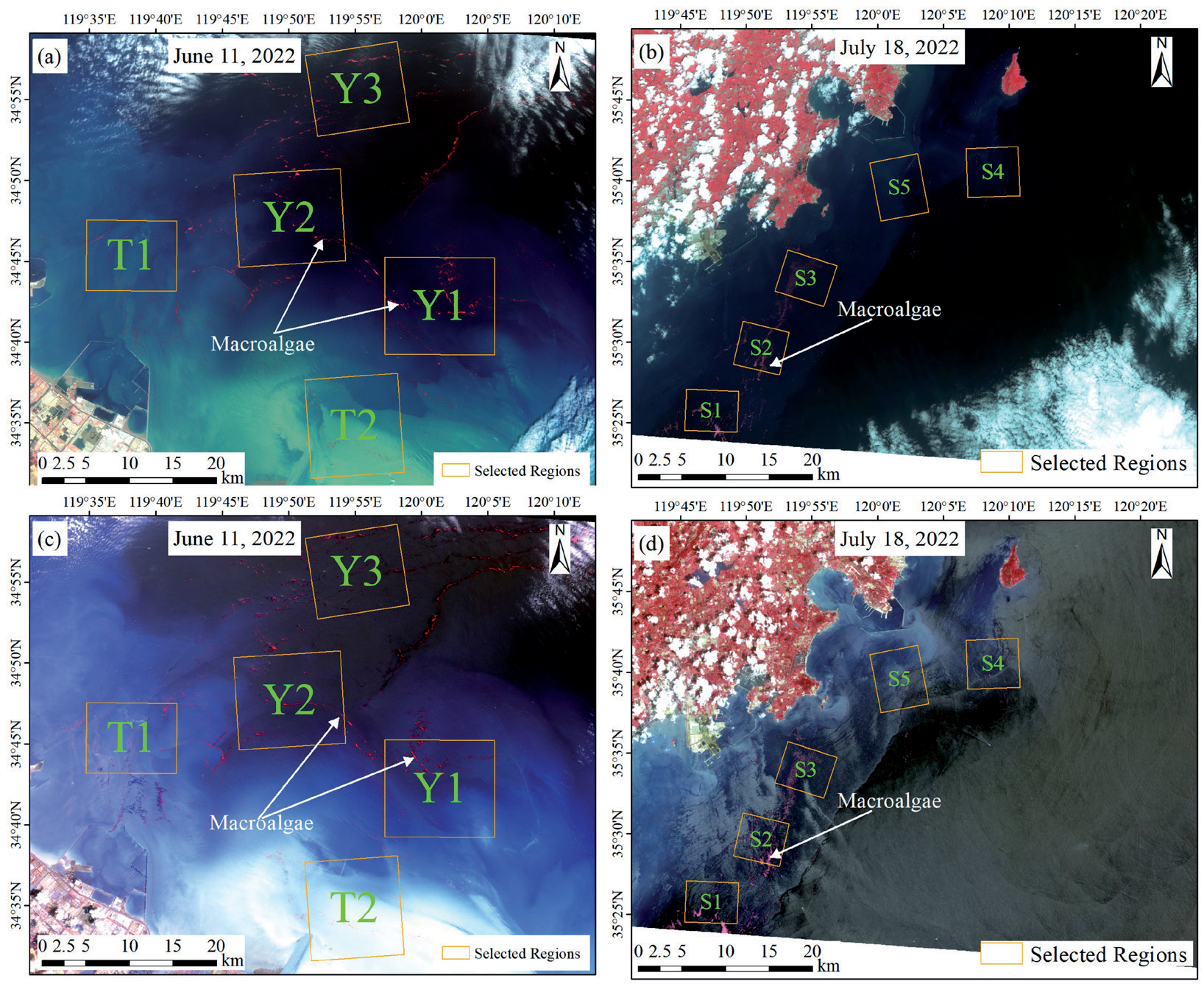
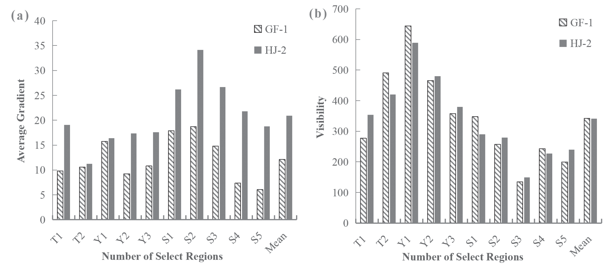
Fig. 4.
Comparison of MAB monitoring results of HJ-2 and GF-1. a) and b) show the spatial distribution of the floating macroalgae monitored by remote sensing images and the locations of the similar patches that were selected, and c) shows a comparison of the coverage area of the selected patches.
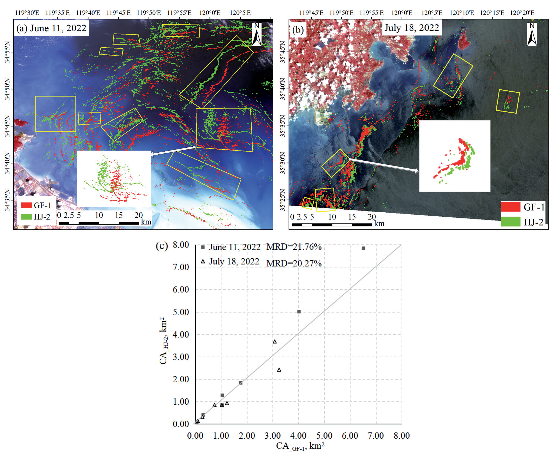
Fourteen pairs of macroalgae with the same or similar distribution were selected to investigate consistency in the retrieved macroalgae coverage area. The results showed that the coverage area estimated by HJ-2 was consistent with that estimated by GF- 1. The MRD on 11 June and 18 July 2022 were 2 1.76% and 20.27%, respectively (Fig. 4). The MRD might be smaller if the time interval were smaller. This result shows that the macroalgae monitoring results derived from HJ-2 and GF-1 are close to each other.
Variation in the Area of MABs in the Yellow Sea in 2022
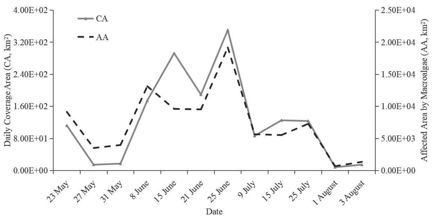
According to the monitoring results from HJ-2 images, the duration of MABs in the Yellow Sea in 2022 was 71 days. Fig. 5 shows the variation in area. The development trend of the CA and AA (Area Affected by MABs, defined in Materials and Methods Section) of MABs was similar to that of previous years, with four stages: emergence, development, outbreak, and dissipation [9]. The maximum values of CA and AA (3.50×10² km2 and 1.92×10⁴ km2, respectively) occurred on the same day (25 June 2022). In the development and outbreak phase (from May 27 to June 25), CA and AA increased by about 11.98 km2/day and 5.59×10² km2/day on average, respectively. In the dissipation phase (from June 25 to August 3), CA and AA decreased by about 8.61 km2/day and 4.57×10² km2/day on average, respectively. Even when CA was relatively small (less than 1.00×10² km2), the AA was higher than 5.00×10³ km2, indicating that the influence of MABs was still serious in the early and late stages of the MABs.
Spatiotemporal Variation and Distribution Density Variation in the Yellow Sea in 2022
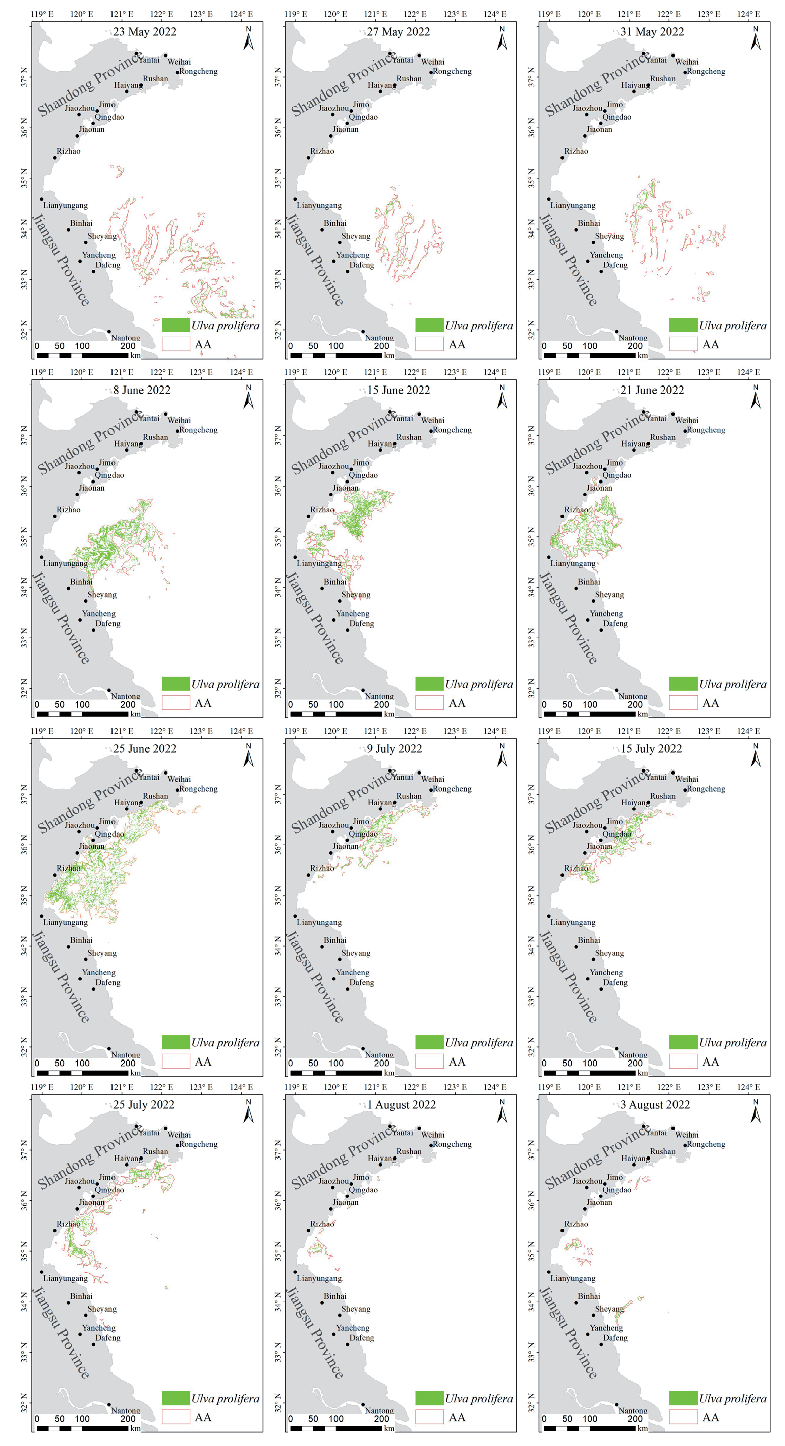
Fig. 6 shows the spatiotemporal distribution map of MABs in the Yellow Sea in 2022, reflecting the distribution and variation of MABs. Macroalgae were found near the Subei Shoal of Jiangsu Province on 23 May 2022. MABs were concentrated in the seawaters near the Subei Shoal until 31 May. After that, MABs began to move north. CA and AA increased to their maximum on 25 June (Fig. 5). During this period, MABs began to affect the offshore waters of the Shandong Peninsula. Then, MABs gradually decreased, and by 3 August, the CA was less than 15.00 km2. At this point, the MABs were at the end of the dissipation phase. During the dissipation phase, MABs were concentrated in the coastal waters of the Shandong Peninsula. After 3 August, macroalgae were not detected in the remote sensing images, indicating that MABs in 2022 were coming to an end.
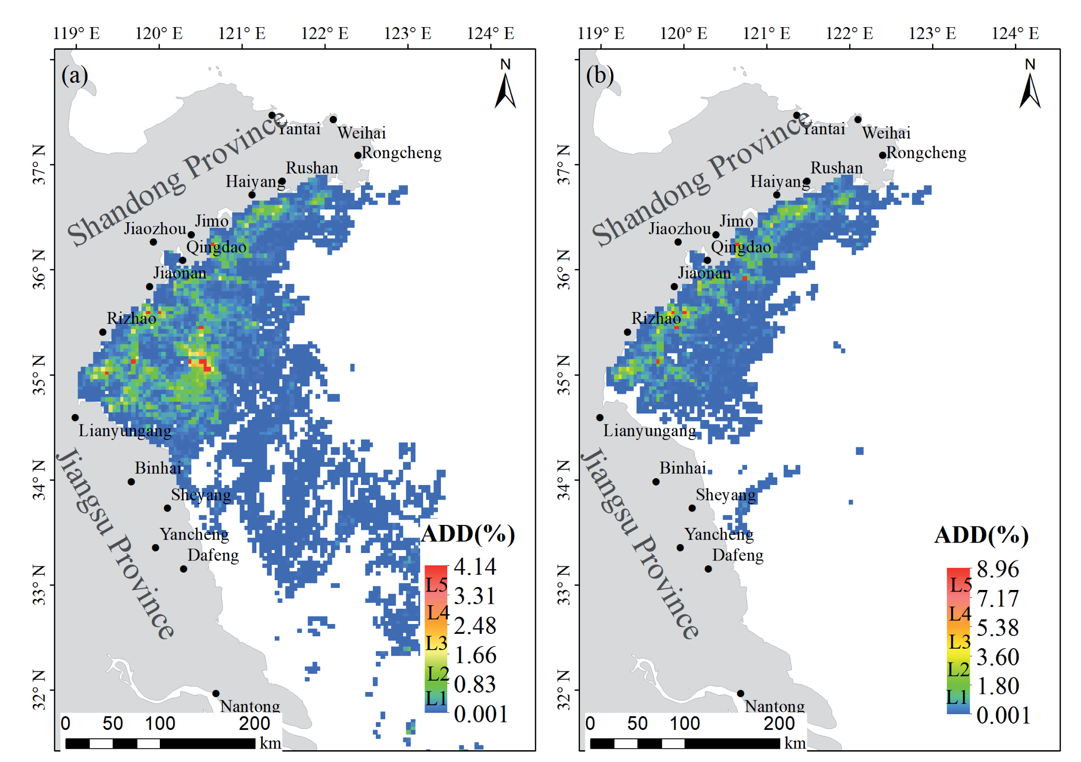
Fig. 7 illustrates the annual distribution density (ADD) of MABs in the Yellow Sea in 2022 during the whole phase (Fig. 7a)) and the dissipation phase (Fig. 7b)). The ADD of the coastal waters of Shandong Peninsula and the central waters of the Yellow Sea was significantly higher than that of other sea areas, indicating that the effect of MABs on these areas was higher than on other sea areas (Fig. 7a)). In particular, the ADD on the coastal waters of Shandong Peninsula was higher than in other sea areas during the MABs dissipation phase, indicating that the effect of MABs on the coastal waters of Shandong Peninsula was more serious (Fig. 7b)).
Discussion
The results obtained in this study would be more compelling if images from a third-party satellite with a higher resolution (e.g., Sentinel-2 images with a spatial resolution of 10 m) or field observation data were incorporated for comparison. However, we were unable to locate GF-1, HJ-2, and Sentinel-2 images that had been captured on the same day, and we could not guarantee that the satellite and field observations coincided spatially due to the floating macroalgae drifting, which made it challenging to obtain field data for comparison. Furthermore, only two simultaneous images were available in this study. Although these images covered different seawater backgrounds and macroalgae aggregation patterns, because remote sensing imaging is inherently complex, an increased number of concurrent image comparisons is needed in future studies to enhance result reliability.
It is undeniable that the HJ-2 satellite has noticeable advantages in MAB monitoring. Combined monitoring using HJ-2, GF-1, and GF-6 enables the dynamic monitoring of MAB with high spatial (16 m) and temporal (1 day) resolutions, thereby mitigating the discrepancy in the estimated MAB area caused by variations in spatial resolution among multiple satellites. This approach enhances the accuracy of quantitative analyses of MABs. In addition, HJ-2 has the ability to detect small patches of Ulva prolifera that may be missed by other satellites with higher temporal resolutions (such as MODIS or GOCI, which have spatial resolutions of 250 m and 500 m, respectively). This enables the more accurate analysis of Ulva prolifera drift speed and drift trajectory prediction.
However, as HJ-2 provides optical images, it is also susceptible to cloud cover and fog, particularly during the occurrence of MABs in the Yellow Sea’s rainy season. In 2022, HJ-2 images of the study area with minimal or no cloud cover were only available for 12 days (Fig. 6). Thus, the limitations associated with optical imagery restrict the availability of data. To enable more frequent dynamic observations, the supplementary use of microwave imaging should be considered due to its ability to penetrate clouds and fog without being significantly affected by them [39, 40]. Furthermore, the imaging principles of remote sensing mean that HJ-2 imagery predominantly shows the characteristics of the sea surface, enabling the effective detection of floating macroalgae. However, its detection accuracy for submerged macroalgae remains relatively low. To enhance the detection accuracy further, field adjustments should be incorporated into the analysis.
Conclusions
In this paper, the macroalgae detection capability of the HJ-2 CCD camera was evaluated by comparing three indicators of the DVI image: average gradient, the macroalgae visibility on the DVI image, and the mean relative difference (MRD) between the macroalgae patch area detected by the GF-1 image and the HJ-2 images. The results showed that the average gradient of the HJ-2 images was slightly better than that of the GF-1 WFV images, and the macroalgae visibility of the HJ-2 CCD images was comparable to that of the GF-1 DVI images. The MRD between them was less than 22%, indicating that the macroalgae detection capability of HJ-2 CCD was the same as that of GF-1 WFV. If HJ-2 could operate with GF-1 WFV and GF-6 WFV, the observation frequency of MABs would be significantly improved. We could accordingly achieve MAB monitoring with fine spatial resolution (16 m) and time resolution (1-2 days) while avoiding the problems of differences in the estimated area associated with using different resolution images.
HJ-2 images with minimal cloud cover from 2022 were selected to monitor MAB. The spatiotemporal variation of MABs in 2022 was analyzed based on three characteristics: macroalgae daily coverage area (CA), the area affected by MABs (AA), and the degree to which MABs were affecting the Yellow Sea, which was represented by the annual distribution density (ADD). The results showed that the spatiotemporal variation of MABs in 2022 was similar to the variation of previous years, encompassing the four typical stages of emergence, development, outbreak, and dissipation. The ADD levels offshore of Rizhao and Lianyungang in the dissipation phase in 2022 were higher than those of previous years. Further research is needed in this regard, along with hydrography data, such as flow field and temperature.

