

Introduction
Tree species diversity plays a crucial role in ecosystems, as it not only enhances the stability of the ecosystem but also effectively resists natural disasters such as pests and diseases. Protecting and restoring tree species diversity has immeasurable value in maintaining the ecological balance of the Earth and promoting sustainable human development [1-3]. Plant species diversity is crucial for enhancing ecosystem services.
The degree of mixed forest, as the core representative of tree species diversity in forest spatial structure, has become an important indicator for evaluating forest diversity in recent years. It quantifies the degree of mutual isolation between tree species in the horizontal direction of the forest stand and is one of the key parameters for describing the spatial structure of the forest stand [5-8]. However, under certain conditions, mixed forests may lead to increased competition among tree species [9-11]. Overall, the construction of mixed forests can effectively promote soil and water conservation, improve soil quality, and enhance biodiversity [12-14]. In addition, mixed forests can also alter the composition and function of fungal communities, which is beneficial for improving soil quality and effectively obtaining tree nutrients [15]. Introducing local nitrogen-fixing broad-leaved tree species into coniferous forests can also improve the chemical stability of soil organic carbon [16], which can affect the cycling of metal elements in forest soils [17, 18]. Overall, mixed forests play an important role in maintaining the health and stability of forest ecosystems.
Natural secondary forest is a type of forest that is naturally restored to its original state after logging or repeated destruction. Its basic structure and original function may have been damaged to a certain extent, and how to improve its mixed value has become a focus of concern for many forest managers [19-22]. Given the uniqueness of natural forests, the current mainstream forest management strategies tend to adopt replanting and selective logging methods. However, optimizing the blending degree of forest stands requires reconstructing the relationships between adjacent trees after each logging to truly reflect the changes in forest spatial structure. However, this dynamism can lead to nonlinearity of the objective function, making traditional mixed integer programming (MIP) no longer able to solve medium to large-scale problems (such as problems with over 50 trees). At present, there are not many reports on how to optimize mixed forests, and the potential for optimizing mixed forests is still unclear [23].
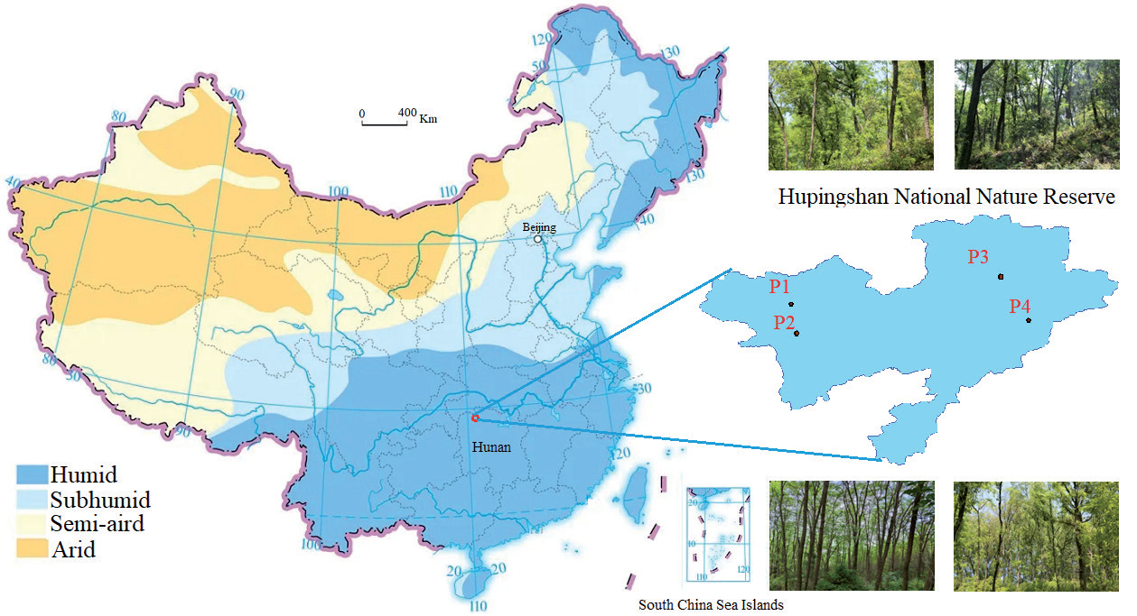
In order to explore the feasibility of the particle swarm optimization (PSO) algorithm in optimizing forest mixing degree, this study takes Hupingshan National Nature Reserve in Hunan Province, southern China, as the research area. The region has a subtropical monsoon climate with an annual precipitation of over 1500 mm, an average annual temperature of 16-18ºC, and a long frost-free period. Select four representative secondary mixed forest stands as research objects. Based on the basic principles of particle swarm optimization, a multi-objective optimization model for forest mixed degree was constructed, attempting to answer the following key questions:
(1) How to quickly and accurately determine the trees to be selected for cutting in the study plot without reducing the number of forest species in the plot in order to improve the blending degree value of the forest stand?
(2) How effective is the particle swarm optimization algorithm in solving the optimization problem of the Stand Mixing Degree?
(3) Is there a linear relationship between the mixed degree value of the forest stand and the selective cutting ratio of the forest stand? What is the optimal selective cutting ratio and the upper limit of the mixed degree value of the forest stand for a certain plot?
Materials and Methods
Study Area and Data Sources
Hunan Hupingshan National Nature Reserve is located in Shimen County, Changde City, Hunan Province, China. It is situated between longitude 110°29′~110°59′ and latitude 29°50′~30°09′. With a total area of 66,568 hectares, it is the largest nature reserve of forest ecosystem in Hunan Province, China. The forest coverage rate is as high as 90.1%, and the vegetation coverage reaches 98.7%. It is one of the few well-preserved areas in subtropical China. To conduct relevant research, four typical natural secondary mixed forests with an area of 20 m × 30 m were carefully selected in the Hupingshan National Nature Reserve as the research objects. The dominant tree species to be studied include Cinnamomum camphora, Acer palmatum, Paulownia fortunei, Pinus massoniana Lamb., etc. (Fig. 1).
In the study area, detailed records were obtained for the number, coordinates, species name, height, diameter at breast height (DBH), and average crown width of trees in plots P1 to P4. The total number of trees ranged from 63 to 84, with average heights between 11.25 m and 13.92 m, average DBH values between 14.26 cm and 18.57 cm, and average Mixing Degrees between 0.37 and 0.54. The dominant tree species and their proportions varied among plots. The basic information regarding the main tree species and their proportions, total number of trees, average tree height, average DBH, and average Mixing Degree in plots P1, P2, P3, and P4 is presented in Table 1.
Methods
Quantification of the Stand Mixing Degree
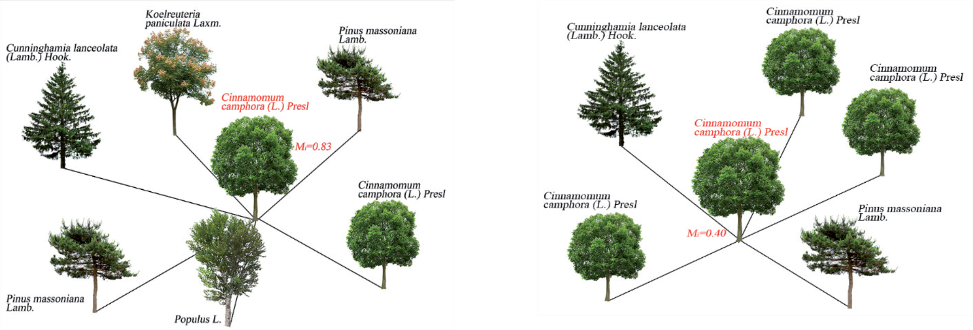
Species Mixture Degree refers to the proportion of neighboring individuals that do not belong to the same species as the target tree among its n nearest neighbors. This metric is utilized to quantify the degree of spatial isolation or mingling among tree species, reflecting the species composition and spatial arrangement (indicating non-homogeneity) within a forest stand. It is mathematically expressed by Equation (1), as referenced in [24, 25].
Mi is the Mixture Degree value of the target tree i, n is the number of neighboring trees of the target tree i, and ϑij is the variable value. When the j-th neighboring tree is of the same species as the target tree i, ϑij = 0; otherwise it is ϑij = 1. For example, the spatial distribution of the target tree with a Mixture Degree of 0.83 and 0.40 is shown in Fig. 2.
The Stand Mixing Degree value is the average of the mingling degrees of all trees, as expressed by Equation (2).
M̅ is the Stand Mixing Degree value, and N is the total number of trees in the forest stand.
Neighboring Tree Selection Scheme
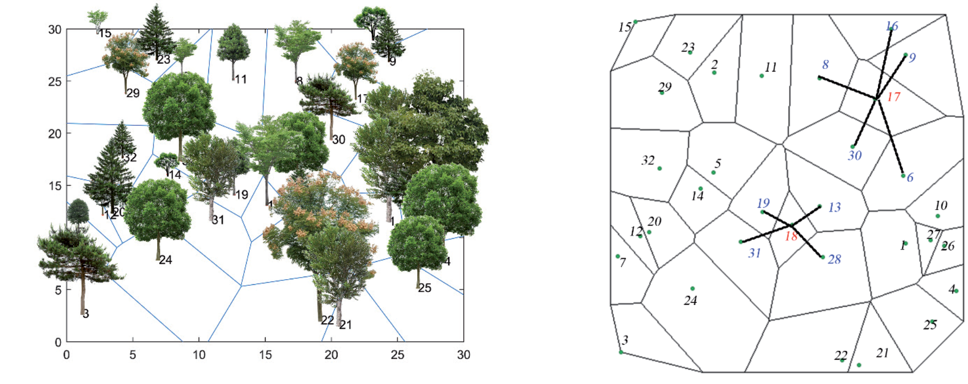
Selecting neighboring trees for a target tree is fundamental to the quantification of the Stand Mixing Degree. The Mixture Degree of the same tree can vary under different neighboring tree selection schemes. Common schemes include the “1+4” theory, the radius R circle theory, and the Voronoi diagram theory [26, 27], with the latter being the most scientific [28]. Therefore, this study employs the Voronoi diagram theory to determine neighboring trees for the target tree. To avoid edge effects, trees with incomplete boundaries in Voronoi diagrams are excluded as target trees but can serve as neighboring trees. For example, trees numbered 15 and 3 are excluded as target trees. The neighboring trees of tree number 17 are {8, 16, 9, 6, 30}, and those of tree number 18 are {19, 13, 28, 31}. The spatial distribution of trees based on Voronoi diagram theory is shown in Fig. 3.
Table 1.
Basic characteristics of forest stands in the study plots.
Mathematical Model for Multi-Objective Optimization of the Stand Mixing Degree
In order to enhance the tree species diversity of the stand, this study is carried out based on the design idea of the maximum upper limit of the Stand Mixing Degree improvement under different selective cutting ratios in the same sample plot. Three optimization objectives are set: (1) To ensure the diversity of tree species in the stand, the number of tree species in the stand after optimization should not decrease. (2) After optimization, the Species Mixture Degree should tend to be as uniform as possible. (3) The Stand Mixing Degree after optimization should increase.
For the convenience of optimization, this paper converts multiple objectives into a single-objective problem using the numerator-denominator method. The basic mathematical model is shown in formulas (3) to (8).
f is the comprehensive objective function (Forest Stand Fitness), Yl is the number of tree species in the forest stand after optimization, Yo is the number of tree species in the forest stand before optimization, flo is the function of the number of tree species before and after optimization, fσt is the standard deviation of the optimized The Stand Mixing Degree, U is the initial set of trees, Z is the collection of selected trees to be selectively cut, z is the total number of trees for selective cutting, N is the initial total number of trees, Mi is the mixed degree value of the i-th tree, P is the selective cutting ratio, M̅ i is the Stand Mixing Degree value after optimization, Nt is the total number of trees after selective cutting.
The Design Concept of the Stand Mixing Degree Optimization Model Based on Particle Swarm Algorithm
The Particle Swarm Optimization (PSO) algorithm was initially proposed by Kennedy and Eberhart [29] and has been widely applied in various fields due to its robust convergence ability in complex solution spaces [30, 31]. Because the optimization problem of mixed forest stands is similar to a highly discrete and spatially complex nonlinear problem, in order to address these challenges, this study introduces three key modifications to the traditional PSO algorithm:
(1) A dynamic search radius mechanism (Equation (13)) was developed to balance the trade-off between exploration and development, and an initial radius of 8 m was determined based on standard forestry practices.
(2) The location update strategy combines Voronoi-based neighborhood analysis (Fig. 4) to limit the search to the tree clusters that are closest to the individual best solution (Equations (14-15)).
(3) A multi-objective fitness function (Equation (3)) was constructed to maximize the forest stand combination (Equation (6)) while minimizing its spatial variance (Equation (5)), ensuring the maintenance of species richness (Equation (4)).
In addition, the initialization parameters of particles are determined based on the size of the forest stand and the intensity of logging (Equations (9-12)), which enables dynamic exploration of datasets of different sizes in the study plot. Through novel configurations of initial position, particle velocity, quantity, velocity update rules, and position adjustment strategies, the complex optimization problem of the Forest Stand Mixing Degree is transformed into an optimization problem of the PSO algorithm, achieving effective optimization of the Forest Stand Mixing Degree.
Initialization
(1) Initial number of particles
The initial particle count in Particle Swarm Optimization (PSO) constitutes a pivotal parameter. An insufficient number of particles may lead the algorithm into local optima. Conversely, an excessive number can enhance the algorithm’s convergence and global search capabilities, yet it also augments computational complexity and runtime, thereby slowing down the algorithm’s convergence rate. Drawing upon the unique characteristics of the forest mixed-degree optimization problem and through extensive experimental validation, this article establishes the initial particle count as formulated in Equations (9) and (10).
INI is the initial number of particles, N is the total number of trees in the forest plot, Nc is the number of trees that need to be selectively cut during the process of optimizing the Forest Stand Mixing Degree, using the standard rounding scheme. p is the proportion of selective cutting, and the range of values generally does not exceed 25%; ⌈ ⌉ is the symbol for rounding up.
(2) Particle dimensions
The particle dimension corresponds to the length of each particle’s solution vector, reflecting the complexity and structure of the problem’s solution space. According to the design concept of the particle swarm optimization algorithm presented in this article, since each particle represents a feasible solution in the optimization process of the Stand Mixing Degree, the particle dimension is equivalent to the number of trees selected for cutting. This value is specified in Equation (11).
d is the dimension of particles, and Nc is the number of trees that need to be selectively cut during the optimization process of the Stand Mixing Degree.
(3) Particle initialization value
The initial value of a particle is a set of random and unique tree numbers with a length of d. For example, the initial value x0id of the particle i is shown in Equation (12).
In the above equation, x0id represents the initialization value of the particle i composed of d random numbers from tree numbers 1 to N, and rand() is the random value function.
Particle Velocity Update Strategy
The mixed degree of some secondary forests in southern China shows a clear trend of low aggregation. In order to solve the problem of clustering distribution of trees with low mixed degree values, the algorithm dynamically adjusts the priority of adjacent trees within the neighborhood search radius based on spatial distance during the optimization process, achieving a breakthrough in spatial pattern homogenization. By removing redundant individuals of the same tree species, the proportion of neighbors of different tree species around the target tree species is effectively increased, thereby improving the overall mixed degree value of the forest stand. Based on the observation that “if a certain tree is harvested, its neighboring trees are more likely to become the target of harvesting”, this study introduces the particle search radius R in the particle swarm optimization (PSO) process. R defines the range of the particle’s next search space and decreases with increasing iteration times. To improve the accuracy and efficiency of the particle swarm optimization algorithm, it is stipulated that when selecting a tree for logging, all trees within a circular area with a radius R centered on the tree should be considered in the next search for the optimal solution. The specific definition of the search radius R is shown in Equation (13).
R is the search radius during the particle optimization process. rmax is the initial search radius of the particle, which is 8 m in this text. tag is the number of cycles.
Particle Position Update Strategy
According to the design concept that any particle represents a feasible solution in the optimization process of the Stand Mixing Degree, assuming that the historical local optimal value of particle i in the t round is pbesti (the set composed of selected tree numbers) and the global optimal value is gbest, based on the updated particle velocity scheme mentioned above, taking the positions of each tree in pbesti and gbest as the center, the sets of all trees within a circular area with radius R are Dit and Ft, respectively. Therefore, the search space Uit+1 for the optimal solution of particle i in the t+1 round is defined as the local optimal solution(pbesti), global optimal solution(gbest), and the union of sets Dit and Ft of particle i in the t round (Equation (14)). Then, d trees are randomly selected from Uit+1 as the positions of particle i in the t+1 round, as shown in Equation (15).
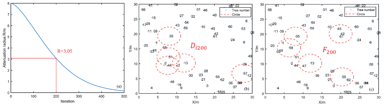
In order to clarify the update scheme of particle position, assuming that the individual optimal solution vector of particle i in the 200-th round is pbesti = {13,35,44,51,57}, the global optimal solution is gbest = {13,35,42,55,58}, and the initial radius is rmax = 8m. According to formula (13), it can be seen that R = 3.06m, so the values of R, Di200, F200, Ui201, and xid201 for particle i in the 201-th round are shown in Fig. 4. Ui201 = {1,2,12,13,16,26,35,42,44,45,47,51,55,57,58,61,62} Di200 = {2,44,47,26,12} F200 = {45,61,1,16,47,62} xid201 = rand(Ui201, d)
The Execution Process of the Algorithm
The execution process of the algorithm follows steps 1 through 4. The specific steps are as follows:
Step 1: Initialization
a) Project all the trees in the sample plot forest onto a two-dimensional plane based on their geographical coordinates. Each tree is represented by a weighted point, which encapsulates the tree’s type, location, height information, etc. These weighted points collectively form the solution space for the particle swarm algorithm (PSO) to search for optimal configurations or solutions.
b) Generate the number of initialization particles INI according to formulas (9) and (10); Determine the particle dimension d according to formula (11); Generate particle initialization value xid0 according to formula (12); According to formula (13), the particle initialization speed and update speed are determined, which are represented by the search radius R in this article.
Fig. 4.
Case study of particle i’s search radius parameters R, Di200, F200 values during optimization.
c) Set the initialization values for parameters such as the maximum number of particle cycles k, the historical individual optimal solution pbesti and historical optimal position li of particle i, the global optimal solution gbest and global optimal position L, and the maximum search range.
Step 2: Evaluation Stage
Calculate the fitness value fit of particle i(i∈1, INI) in the t(t∈(1, k)) round based on xidt and formulas (1) to (8) to evaluate the quality of particle i. The initial fitness value of the forest stand is the fitness value f without selective cutting, with the goal of maximizing the comprehensive fitness of the forest stand (f) under a certain proportion of selective cutting.
Step 3: Update Phase
a) Update individual optimal values
Compare the current fitness value fit of particle i with the historical optimal fitness value pbesti. If the current fitness value is better (fit >pbesti), update the historical best fitness value and historical best position of particle i, so that pbesti = fit, li = xidt i(i∈1, INI).
b) Update the global optimal value
Find the globally optimal fitness value gbestt = Max(pbesti) i∈1, INI and its corresponding position Lt among all particle local optima, update gbest and L, and let gbest = gbestt, L = Lt.
c) Update the velocity and position of particles
Due to the particularity of optimizing the Forest Stand Mixing Degree, in order to prevent the algorithm from entering local optima, this paper sets the weights of each individual and global convergence radius R in the particle swarm to 1. It updates the search radius R and next round position xidt+1 of each particle according to formulas (13) to (15).
Step 4: Iteration and Termination
If the algorithm reaches the maximum number of iterations k, it ends and outputs the global optimal solution gbest and the set of tree numbers L that are for selective cutting. Otherwise, it returns to Step 2 to continue iteration.
Results
To evaluate the optimization effect of the particle swarm algorithm on the Forest Stand Mixing Degree, this study selected four natural secondary mixed forest plots (P1, P2, P3, P4) of 20 m × 30 m in Hupingshan National Nature Reserve, Hunan Province, for testing and analysis. Three selective cutting ratios ‒ 5%, 10%, and 15% ‒ were applied to each plot. The relevant parameter settings for the experimental operations are detailed in Table 2. Note that, given the characteristics of intelligent algorithms in the optimization process, the optimal values of all indicators in the article are defined as the relative optimal values within a specified number of cycles.
Number of Selectively Logged Trees and Their Spatial Distribution
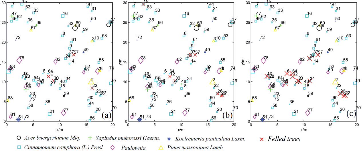
Based on the algorithm’s output, the “optimal” trees for selective cutting in plots P1, P2, P3, and P4 can be identified. For instance, under a 5% selective cutting ratio, the selected tree numbers in plot P1 are 12, 22, 30, and 57, while those in plot P2 are 27, 30, 10, and 3. The detailed tree numbers for each plot under different selective cutting ratios are provided in Table 3. Generally, trees with lower Mixing Degrees are more likely to be selected for cutting. In plot P1, for example, under a 15% selective cutting ratio, the selected trees have relatively low Mixing Degrees, ranging from 0 to 0.4 with an average of 0.16. Specifically, 26.67% of the selected trees have a Mixing Degree of 0, 20% have a Mixing Degree of 0.17, and 73.33% have a Mixing Degree below 0.29. However, the selected trees vary with different selective cutting ratios. The spatial distribution of selected trees in plot P1 under various cutting intensities is illustrated in Fig. 5.
Changes in Forest Stand Fitness
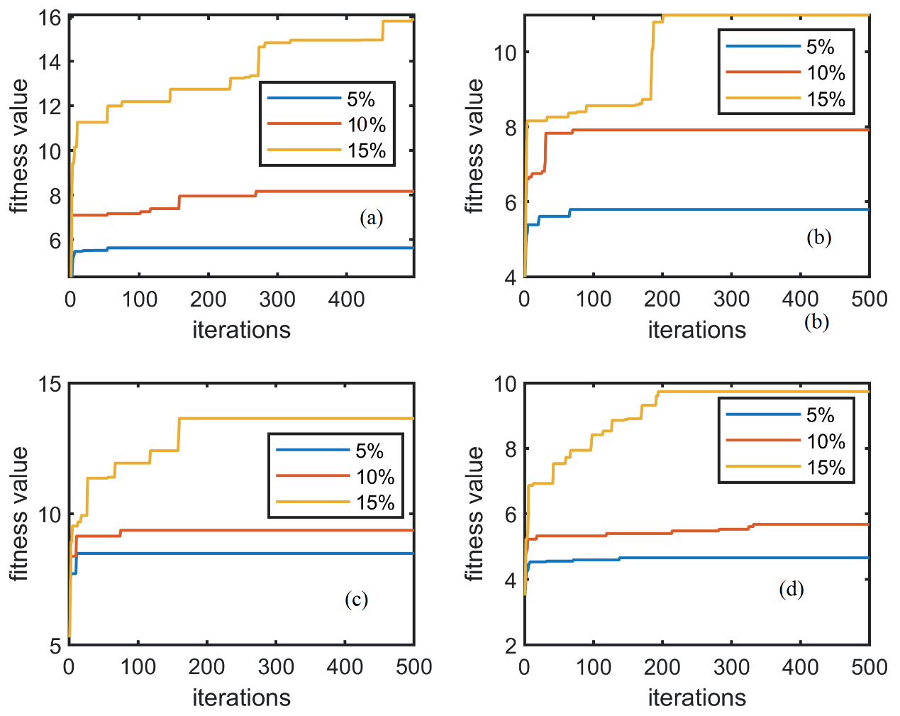
The research results show that under different logging intensities (5%, 10%, 15%), the fitness values of all plots are significantly improved, proving the feasibility of using this algorithm to optimize forest stand combinations. However, the growth rate of fitness values varies depending on the cutting strength. As the cutting intensity increases, the growth rate also increases, although the growth curve is not strictly linear (Fig. 6). For example, in plot P1, when the cutting intensities are 5%, 10%, and 15%, respectively, the fitness values increase from the baseline of 4.12 to 5.63, 8.17, and 15.87. In plot P2, the fitness values increased from 3.99 to 6.75, 7.92, and 10.98, while in plot P3, the fitness values increased from 5.29 to 8.50, 9.38, and 13.64 (Table 4). These results indicate that moderate selective logging can improve the overall adaptability of forest stands.
Table 2.
Setting of some experimental parameters.
Table 3.
Optimal tree numbers for selective cutting in plots at different ratios.
Changes in Forest Stand Mixing Degree
The mixed degree value of forest stands is a key indicator for evaluating the diversity and spatial pattern of tree species in forest ecosystems, which shows significant dynamic changes after selective logging optimization. In the studies of plots P1 to P4, although there were fluctuations in the particle swarm optimization process, the overall trend was upward, especially at a cutting intensity of 15%, where this improvement was most significant (Fig. 7). For example, under selective logging ratios of 5%, 10%, and 15%, the mixing degree values of the P1 plot increased by 15.22%, 30.43%, and 52.17%, respectively. Similarly, the growth rates of the mixed degree values in plot P2 were 20.45%, 22.73%, and 31.82%, respectively. The mixed degree values in the P3 chart increased by 18.87%, 22.64%, and 35.85%, respectively. The mixed degree value of the P4 plot also achieved significant growth, with improvement rates of 13.04%, 21.74%, and 47.83%, respectively (Table 5). Selective logging not only promotes tree species diversity but also optimizes the spatial distribution of tree species, enhances the stability and resistance of forest ecosystems, and provides a scientific basis for sustainable forest management.
Table 4.
Forest stand fitness changes with selective cutting.
Changes in the standard deviation of the Stand Mixing Degree
After implementing the selective logging optimization strategy, the standard deviation of the mixed degree in the four experimental forest plots significantly decreased. For example, in plot P1, under selective cutting of 5%, 10%, and 15%, the standard deviation decreased by 18.18%, 36.36%, and 63.64%, respectively, and plot P2 decreased by 27.27%, 36.36%, and 54.55%; plot P3 decreased by 30.00% and 50.00%, respectively; and the P4 plot decreased by 8.33%, 16.67%, and 41.67% (Table 6). These results indicate that selective logging optimization leads to a more uniform degree of forest mixing, with an increase in the number of trees with a mixing degree between 0.4 and 0.8. The proportion of individual plants with a low mixing degree, especially those with a mixing degree of 0, significantly decreased. This indicates that the distribution of tree species is more reasonable, and the stability and biodiversity of the ecosystem are enhanced.
Table 5.
Forest stand Mixing Degree changes with selective cutting.
Fig. 7.
Trends in forest stand mixing degree during the algorithm optimization process. (a), (b), (c), and (d) depict the changing trends of Forest Stand Mixing Degree in plots P1, P2, P3, and P4, respectively, throughout the algorithm optimization process.
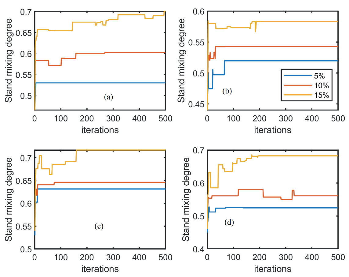
Table 6.
The standard deviation of the stand Mixing Degree changes with selective cutting.
Changes in Tree Species Number and Proportion
The optimization results indicate that the number of tree species in plots P1, P2, P3, and P4 remained unchanged under selective cutting ratios of 5%, 10%, and 15%, but the proportion of dominant tree species changed, meeting the expected target requirements of the particle swarm algorithm (Table 7). For example, in plot P1, the initial proportion of Acer buergerianum was 3.6%. Under selective cutting ratios of 5%, 10%, and 15%, its proportion increased to 3.75% (+0.15%), 3.95% (+0.35%), and 4.23% (+0.63%), respectively. The proportion of Sapindus mukorossi increased from 4.76% to 5.00% (+0.24%), 5.26% (+0.50%), and 5.63% (+0.87%), respectively. In contrast, the Cinnamomum camphora proportion decreased significantly from 64.29% to 61.25% (-3.04%), 59.21% (-5.08%), and 56.34% (-7.95%). After optimization, the overall types of trees in each plot remained unchanged, despite some changes in proportions (Table 7).
Table 7.
Changes in tree species number and proportion in plots P1 to P4.
Discussion
Response Analysis of the Stand Mixing Degree Under Different Selective Cutting Ratios
As an important indicator of forest spatial structure, the degree of mixed forest plays a crucial role in measuring forest diversity. Most researchers now consider using selective cutting to improve forest spatial structure and increase the degree of mixed forest [32, 33].
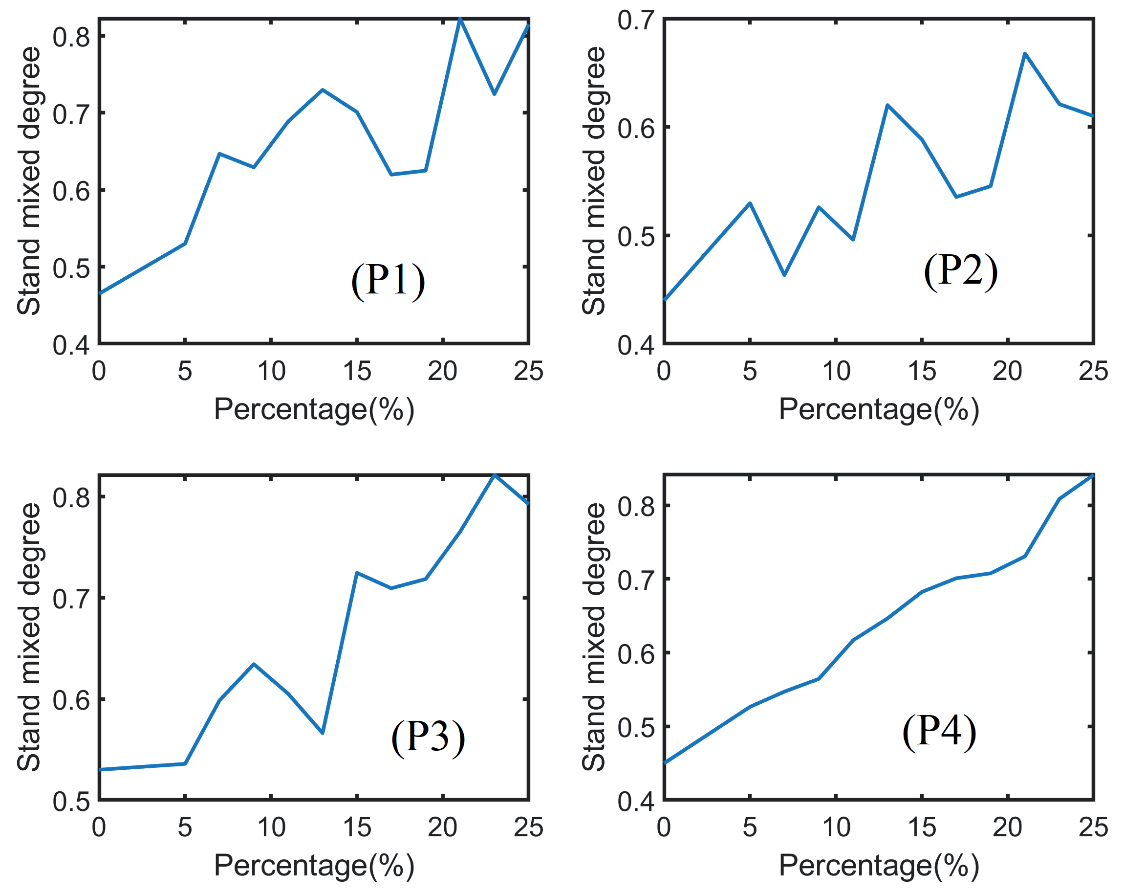
Selective cutting can improve the Mixing Degree of forest stands, but the response of the Mixing Degree to different selective cutting ratios is not clear. To study the variation of the Forest Stand Mixing Degree with selective cutting ratio, this paper investigated selected plots P1, P2, P3, and P4 at 2% intervals within an optimal range of 5% to 25%. Results showed that the optimal Mixing Degree values and corresponding selective cutting ratio for the four plots were: P1 (0.82, 21%), P2 (0.66, 21%), P3 (0.82, 23%), and P4 (0.84, 25%). Overall, the Mixing Degree values of plots P1 to P4 increased with increasing selective cutting ratios up to 25%, but the trends varied and fluctuated, without showing strong linear changes (Fig. 8).
Specifically, plot P1 had a relatively concentrated tree species distribution and weak mixing, which improved as the selective cutting ratio increased, reaching a maximum Mixing Degree of 0.82 at 21%. Plot P2 also showed an upward trend, with a maximum Mixing Degree of 0.62 at 23%, although the increase was smaller than in P1. Plot P3’s Mixing Degree remained relatively stable but generally increased with higher selective cutting ratios. Plot P4 exhibited a weak linear upward trend, with the most significant change among the plots, reaching a maximum Mixing Degree of 0.84 at 25%. Its tree species composition and spatial distribution pattern were highly sensitive to selective cutting, which strongly promoted mixing.
Despite overall increases in Mixing Degree with higher selective cutting ratios, differences existed among plots. For example, plot P4 showed more significant changes, likely due to its greater sensitivity to selective cutting. Improved mixing can enhance forest community diversity and complexity, thereby increasing ecosystem stability and resistance. However, excessively high selective cutting ratios may cause irreversible damage and reduce ecosystem stability [34]. Therefore, in practice, it is essential to consider the specific conditions of each plot and control selective cutting intensity to achieve sustainable forest management.
Comprehensive Analysis of PSO in the Optimization of Forest Mixing Degree
As a classic global optimization method, Mixed-Integer Programming (MIP) typically achieves implicit enumeration and converges to the absolute optimal solution through techniques such as branch-and-bound and cutting planes [35, 36]. In this study, the dynamic Voronoi neighborhood model requires reconstructing topological relations after forest harvesting, leading to strong nonlinearity in the objective function. As a result, the implicit enumeration of traditional MIP cannot exclude invalid branches, and solution time may grow exponentially with the increase of problem scale [37].
To verify the effectiveness of Particle Swarm Optimization (PSO) in terms of solution quality and time efficiency, this paper compares MIP (full combinatorial enumeration) with PSO in 10 small-scale plots with 30 trees each (LS1-LS10). In 4 medium-scale plots with 79-200 trees (MS1-MS4) and 2 large-scale plots with 350-499 trees (HS1-HS2), PSO is compared with Genetic Algorithm (GA), Artificial Bee Colony (ABC), and Differential Evolution (DE) algorithms to evaluate the solution quality of PSO at different scales. The specific experimental design is shown in Table 8 (the cutting ratio is 15%). To minimize random impacts on intelligent algorithms and enhance result reliability, this paper executed the algorithm 30 times per experimental plot and used the average values as the analytical basis for comparison.
The research results indicate that the small-scale PSO strictly converges to the absolute optimal solutions of the MIP (Mixed-Integer Programming) in 70% of the plots (LS1, LS2, LS3, LS5, LS6, LS7, LS9), demonstrating full equivalence to the exact algorithm. This suggests that it possesses the capability to solve for global optimal solutions in most scenarios. For the remaining 30% of the plots (LS4, LS8, LS10), the maximum relative error between the PSO solutions and the MIP optimal solutions is only 1.47% (LS8: 0.5240 vs. 0.5318) (Table 9).
Based on the initial values, the MIP algorithm achieves an average improvement of 23.67%, while the PSO algorithm achieves an average improvement of 22.89%, with a difference of only -0.78%. The paired t-test shows that the mean difference between the PSO solutions and the MIP optimal solutions is not statistically significant (p = 0.14) (Table 10), proving that the optimization capability of PSO is essentially comparable to that of the exact algorithm as a whole.
Table 9.
Performance comparison between MIP and PSO algorithms.
The average running time of the MIP algorithm is 239.67 seconds, while that of PSO is only 2.70 seconds, representing an efficiency improvement of approximately 88.8 times (Table 9). Notably, the speed difference in Plot LS7 reaches 137 times (MIP: 234.63 seconds vs. PSO: 1.71 seconds), highlighting the overwhelming advantage of PSO in computational efficiency.
The standard deviation of PSO running time is 0.24 seconds, which is only 2% of that of MIP (12.14 seconds), indicating its stable convergence across different problem structures and avoiding the time fluctuations of the exact algorithm caused by problem complexity.
Based on the paired t-test (t = -1.62, p = 0.14) and Wilcoxon test (W = 0, p = 0.17), both tests indicate that there is no significant difference in solution quality between PSO and MIP when solving the stand mixing degree optimization problem in small-scale scenarios. In contrast, the t-test for the average computation times between the two shows a highly significant difference (p<0.001) (Table 10).
Table 10.
Comparison of statistical test results between MIP and PSO.
Table 11.
Optimization efficiency in medium-scale problems.
Table 12.
Optimization efficiency in large-scale problems.
In the four medium-scale plots (79-200 trees, MS1-MS4), PSO showed no statistically significant difference in the relative optimal values for stand mixing degree optimization compared with GA (U = 22, p = 0.08) and ABC (U = 18, p = 0.11), but exhibited a highly significant difference from DE (U = 10, p<0.01). The median optimal value of DE was 5.08% lower than that of PSO (95% CI: 4.21%-5.93%).
No significant difference was found in convergence time between DE (68.82±28.31 s) and PSO (84.84±32.56 s) (U = 20, p=0.07), whereas PSO was significantly faster than both GA and ABC (all p<0.01). Notably, the median computation time of GA (180.44 s) was 2.13-fold that of PSO.
PSO required significantly fewer convergence iterations (211.75±38.62) than GA and ABC (all p<0.01) but showed no significant difference from DE (136.50±45.71) (p = 0.06), suggesting that DE may trade solution quality for speed by reducing iteration counts, as shown in Table 11.
In two large-scale plots (350-499 trees, HS1-HS2), PSO and GA exhibited comparable average improvement rates (12.45% vs. 12.30%), with PSO slightly outperforming GA in Plot HS2 (16.17% vs. 16.04%), which demonstrates PSO’s superiority in convergence precision for high-complexity problems. DE achieved only 5.47% average improvement, significantly lower than other algorithms, indicating its limited global search capability (Table 12).
The average computation time of PSO (411.25 seconds) was approximately 41.5% that of GA (991.95 seconds) and 50.9% that of ABC (807.46 seconds), highlighting its remarkable efficiency advantage. Although DE’s average time (483.4 seconds) was comparable to PSO, its inferior solution quality suggests that this may be attributed to premature convergence (e.g., only 53 iterations in Plot HS1).
PSO required fewer average iterations (384.5) than GA (442) and ABC (433.5), yet significantly more than DE (114.5). This indicates that PSO strikes a better balance between rapid convergence and avoidance of premature convergence compared to GA/ABC and is less prone to local optima than DE.
Overall, in small-scale problems, PSO (Particle Swarm Optimization) not only achieves solution quality close to that of MIP (Mixed-Integer Programming), but also demonstrates extremely high time efficiency and strong algorithmic stability. In medium-to-large-scale problems, by balancing the number of iterations and convergence accuracy, PSO exhibits stronger global search capability in complex-scale problems. Compared with evolutionary algorithms such as GA (Genetic Algorithm) and ABC (Artificial Bee Colony), PSO has superior time efficiency under the premise of comparable solution quality. Compared with the DE (Differential Evolution) algorithm, PSO significantly outperforms DE in solution quality and avoids “premature convergence”.
Conclusions
This study constructed a natural secondary forest blending optimization model based on the particle swarm optimization (PSO) algorithm. It verified the optimization efficiency of PSO under different logging intensities (5%, 10%, 15%) using the forest stands in Hupingshan Nature Reserve, Hunan Province, as the object. The main conclusions are as follows:
(1) With the increase of logging intensity, the forest mix shows a nonlinear increase (31.82%~52.17% at 15% intensity), and the spatial distribution uniformity of tree species is significantly improved. PSO optimization did not reduce the number of tree species but adjusted the proportion of dominant tree species reasonably, confirming the feasibility of optimizing spatial structure while maintaining biodiversity.
(2) In small-scale scenarios, compared with mixed integer programming (MIP), PSO reduces the running time by 98.8% (2.70 vs. 239.67 seconds), 70% of the plots converge to the global optimal solution, and the maximum relative error of the remaining plots is only 1.47%. On a medium to large scale, compared with the genetic algorithm (GA) and artificial bee colony algorithm (ABC), PSO has shortened the convergence time by 41.5% to 50.9% and reduced the number of iterations by 21.3%. The quality of the solution is comparable to traditional algorithms, but it is more efficient.
(3) There is no strict linear relationship between the degree of mixing and harvesting intensity, and the optimal harvesting intensity varies depending on forest characteristics (21%~25%). In practical management, it is recommended to control the logging intensity to ≤ 25% and prioritize the logging of trees with a mixing degree ≤0.4 to balance structural optimization and ecological stability.