

Introduction
Due to swiftly accelerating economic growth, air pollution is currently a global public health issue. The natural environment, public health, and economic development are all impacted by air pollution. According to a meta-analysis, cardiovascular disease can increase by 11% on average with long-term exposure to PM2.5 [1]. Over a nine-year follow-up period, a 10% increase in cardiovascular mortality was linked to an increase in PM2.5 exposure in a large cohort aged 50-71 from six U.S. states and two metropolitan regions [2].
As a result, techniques for decision-making and analysis based on models may be created to enhance the creation of air protection plans [3]. When developing air pollution models, two basic methods are often employed: data-driven or empirical modeling and theoretical or deterministic modeling. Theoretical models that are often employed include Community Multiscale Air Quality (CMAQ) [4, 5] and Gaussian diffusion [6]. Air pollution forecasting has made extensive use of classical data-driven models such as the Autoregressive Integrated Moving Average (ARIMA) model [7], Support Vector Machine (SVM) [8, 9], Long Short-Term Memory (LSTM) [10, 11], and Bidirectional Long Short-Term Memory (Bi-LSTM) [12, 13]. Due to its great approximation capability, the PWA (Piecewise Affine) model is a crucial data-driven technique that has attracted a lot of attention and is already being utilized to solve difficult issues in simulation, prediction, and system analysis [14]. Typical application fields of PWA models are providing solutions for vehicle powertrains [14-17], robotics [18], power and energy [19], industry production processes [20-22], and rainfall runoff [23]. Also, the PWA modeling method was adopted for motion segmentation in computer vision [24, 25]. More details about applying PWA models can be found in [14]. By dividing the scheduling space into polyhedral convex regions and creating local models, the PWA model is developed. Partitioning regression space, estimating partition borders, and parameterizing each affine sub-model are typical processes involved in the discovery of PWA models [26]. The challenge of identifying PWA models is often regarded as difficult and is NP-hard [14]. The connection between identification and the classification problem is a major source of difficulty [27]. Numerous techniques have been presented in the past for identifying PWA models. It can provide a model with similar training data, which shortens the training period and increases generalizability. It is possible to estimate the sub-model parameters concurrently or later.
This work focuses on the identification of the PWA model with optimum model order selection using hierarchical clustering. The BIRCH (Balanced Iterative Reducing and Clustering using Hierarchies) technique has garnered a lot of attention in the past several decades as an effective agglomerative hierarchical clustering algorithm. However, clusters with arbitrary forms or changeable volumes should not use this approach [28]. This study introduces an additional phase to BIRCH, whereby partitions with the closest distances are merged until the desired number is reached. Next, the suggested modeling approach is used to forecast Shenyang, China’s air pollution. The proposed method is broad and might be extended to include different kinds of models. The following are this paper’s primary contributions: – To forecast air pollutants, a data-driven PWA model
is presented. This model is defined by dividing the
scheduling space into local regions. – A hierarchical clustering-based method is adopted
for the identification of the PWA model, and the
optimization methodology estimates the model order
and parameters. – The performance of the proposed model is compared
with the baseline models, and the proposed method
is used to forecast air pollution in Shenyang.
Materials and Methods
Study Area
Shenyang, the largest city in northern China, serves as both the physical and transportation core for Northeast Asia and a key hub for the Belt and Road initiative, which connects the region to Southeast and Northeast Asia. Plains and mountains make up the majority of the landscape of this hilly area, which is situated in the southeast. Shenyang has four different seasons and a broad variety of temperatures due to its temperate, subhumid continental environment. The yearly average temperature ranges from 6.2 to 9.7ºC, with considerable seasonal variations. Summer winds are generally southwest and northerly, winter winds are generally north, and spring winds are frequently southwest and northerly. Shenyang saw annual wind speeds ranging from 2.8 to 4.4 m/s, with springtime increases and summertime decreases [29]. The location of Shenyang in China is shown in Fig. 1.
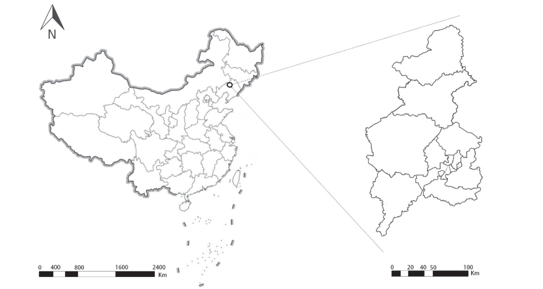
Transportation, central heating, and industrial activity are the key factors influencing Shenyang’s air environment. Since the early days of the creation of New China, Shenyang, one of the first heavy industry bases in China, has established numerous heavy industry production businesses with a solid industrial basis. Its industrial structure is primarily responsible for the high coal use. For instance, in 2016, there was a significant increase in the amount of coal consumed overall – roughly 33 million tons – compared to the national average, which is much lower. Meanwhile, the share of renewable energy was less than 13%. Consequently, because of coal-based consumption, particulate matter (PM) is Shenyang’s main source of air pollution; the city’s annual PM2.5 and PM10 daily exceed rates are 12.1% and 7.7%, respectively. Wintertime coal-burning heating raises PM2.5 and PM10 levels, which leads to extreme pollution. The highest monthly average mass concentrations of PM2.5 were seen in March and February, while the lowest were observed in August.
Data
As was already established, several variables affect air quality, including geography, environmental concerns, social or pollution emissions, and future air pollutants that can be predicted using previous variations. The main factor may be variations in climatic conditions, which have an impact on pollutant concentrations. It has been determined that meteorological data is a crucial input variable for air quality forecasting in statistical and mathematical models. As a result, the recommended forecasting models use meteorological and air pollution data as training sets. The two aspects that make up the datasets used in this study are meteorological variables and factors related to air quality. This contribution combines hourly data to train and assess the PWA air pollution forecasting model. Air pollutants, temperature, humidity, air pressure, dew point, and wind direction/ speed are among the overserved data sets.
Method
The PWA model with hierarchical clustering-based identification is presented in this section.
Model Structure
The PWA model is defined as superposed c local models that explain the MISO (Multiple-Input-Single-Output) system. The predictor of air pollution in this research is the PWARX (Piecewise AutoRegressive eXogenous) model, which has an interpretable nonlinear structure [30]. The model is defined as:
with the regressor:
Where na and nb are model orders, respectively,
Data Processing
The dataset’s outliers and missing data will be handled first. Subsequently, the correlation analysis is carried out to choose pertinent attributes for the prediction model. Pearson’s correlation coefficient (PCC), a commonly used statistical indicator to assess and investigate the degree of correlation between variables in practice, is used to quantify the correlation among characteristics. In time series data, Pearson’s correlation coefficient generally explains the degree to which the goal variable (y) and the input variable (x) correlate over a certain period. The target variable y in this study reflects the measured value of air pollution, whereas the input variables represent the inputs to the PWA model. The following formula may be used to compute Pearson’s correlation coefficient mathematically:
where x̅ is the average of x and y̅ is the average value of y. With +1 denoting total positive correlation, 0 denoting no connection, and -1 denoting total negative linear correlation between x and y, Pearson’s correlation coefficient is between +1 and -1. A greater correlation coefficient value, which denotes a closer relationship between the detected characteristics, will lead to the selection of additional processing.
Then, to solve the issue of the curse of dimensionality, Principal Components Analysis (PCA) will be utilized. By keeping low principal components and ignoring high-order principal components, PCA can minimize the number of dimensions. Then, low-order components may typically preserve important information. The core principle of PCA is to keep the majority of the data while condensing numerous variables into new, uncorrelated ones. The chosen features should be normalized before PCA dimension reduction since the projection will attempt to mimic any substantial premium that a feature may have in the data after the projection, which may lead to a sizable quantity of missing data.
Clustering Method
Then, the scheduling space will be portioned into local regions using clustering. The “similarity” of the data must be assessed for techniques that rely on clustering. As a common machine-learning approach, clustering is used to categorize the data points of related objects. Hierarchical and partitional clustering are two categories of clustering methods. The goal of partitional clustering is to minimize predetermined criteria for dividing data points into c divisions. Hierarchical clustering applies agglomerative and divisive methodologies to progressively investigate a hierarchy of clusters. Agglomerative techniques combine the nearest clusters repeatedly after collecting clusters from the bottom up. Data points are iteratively split into smaller clusters from the top down. BIRCH performs clustering based on a tree structure, namely the Clustering Feature (CF) Tree, as a common agglomerative clustering technique.
It is observed that in the typical BIRCH algorithm, the shape and size of clusters are determined by the same hyperparameter. However, clusters with arbitrary forms or changeable volumes should not use this approach [28]. A modified version of the BIRCH approach is presented in this study to enhance the performance of irregularly shaped clusters. The second step of clustering refines the first stage using the average linkage, which finds the average distance drs between each cluster pair Cr and Cs:
where nr and ns are the numbers of data points in cluster Cr and Cs, xri, and xsj are the i-th and jth data points in cluster Cr and Cs, dist(xri, xsj) is the distance between xri and xsj. The second step is carried out following standard BIRCH until the required number of clusters is reached.
Estimation of the Order and Parameters of Local Models
Once data points have been clustered using the suggested approach, the values of model parameters are estimated using
To ascertain the model order denoted by na and nb in Eq. (2), the Lasso-regularization is introduced by adding a regularization L1-term in Eq. (5).
where
Experiment
Model Quality Assessment
Three criteria are adopted to assess the quantitative quality of the model in this work. They are the correlation coefficient (R), the mean absolute error (MAE), and the root mean square error (RMSE):
where N is the number of test data, y is the true value,
Data Processing
The proposed approach is used in the experiment to forecast the level of air pollution in Shenyang, based on the previously described technique. In the case study, the period of the model construction is from 2016 to 2018. Correlation analysis is conducted to choose pertinent characteristics based on PCC before determining the suggested PWA model. The feature correlation analysis is displayed in Fig. 2. It is shown that the majority of air pollution features have positive correlations, except O3, which is negatively correlated with other features. In Fig. 2 there is a weaker link between meteorological and air pollution characteristics; all parameters except wind and atmospheric pressure have a negative correlation with air pollutants. As previously mentioned, accuracy may be increased by excluding elements that are uncorrelated or weakly linked. In this work, a threshold of 0.2 is specified, and features with correlation coefficients greater than 0.2 are deemed to be strongly associated.
To get over the dimensionality problem, the PCA approach helped to lower the dimension of the number of selected features. The PCA method result shows that over 90% of the information supplied by the complete features is contained in the first three principal components. Therefore, in addition to the anticipated values, these three principal components, which contain important information from the data, are employed for the prediction of air pollution. PCA has been used to extract.
Results and Discussion
Simulation Results
The proposed model will be used to forecast air pollution. In Fig. 3, the observed data is represented by the blue line, while the PM2.5 forecast made by the PWA model is shown by the red line. The estimate accurately depicts the hourly PM2.5. The model’s forecast and the measurement are rather close, which means that the model can precisely predict PM2.5, according to the testing samples. The correlation coefficient (R) between the measurement and prediction of PM2.5 is 0.9849, indicating that almost 98% of the variation was explained by the model. It is also possible to accurately forecast the majority of peak positions, and the prediction curve closely resembles the observed curve. It shows that significant state changes can be handled by the suggested paradigm. However, as Fig. 3 illustrates, the prediction could not consistently fit the actual data with lower concentration values when PM2.5 is less than 110 μg/m3. On the other hand, greater PM2.5 values may be predicted with accuracy by the PWA model.
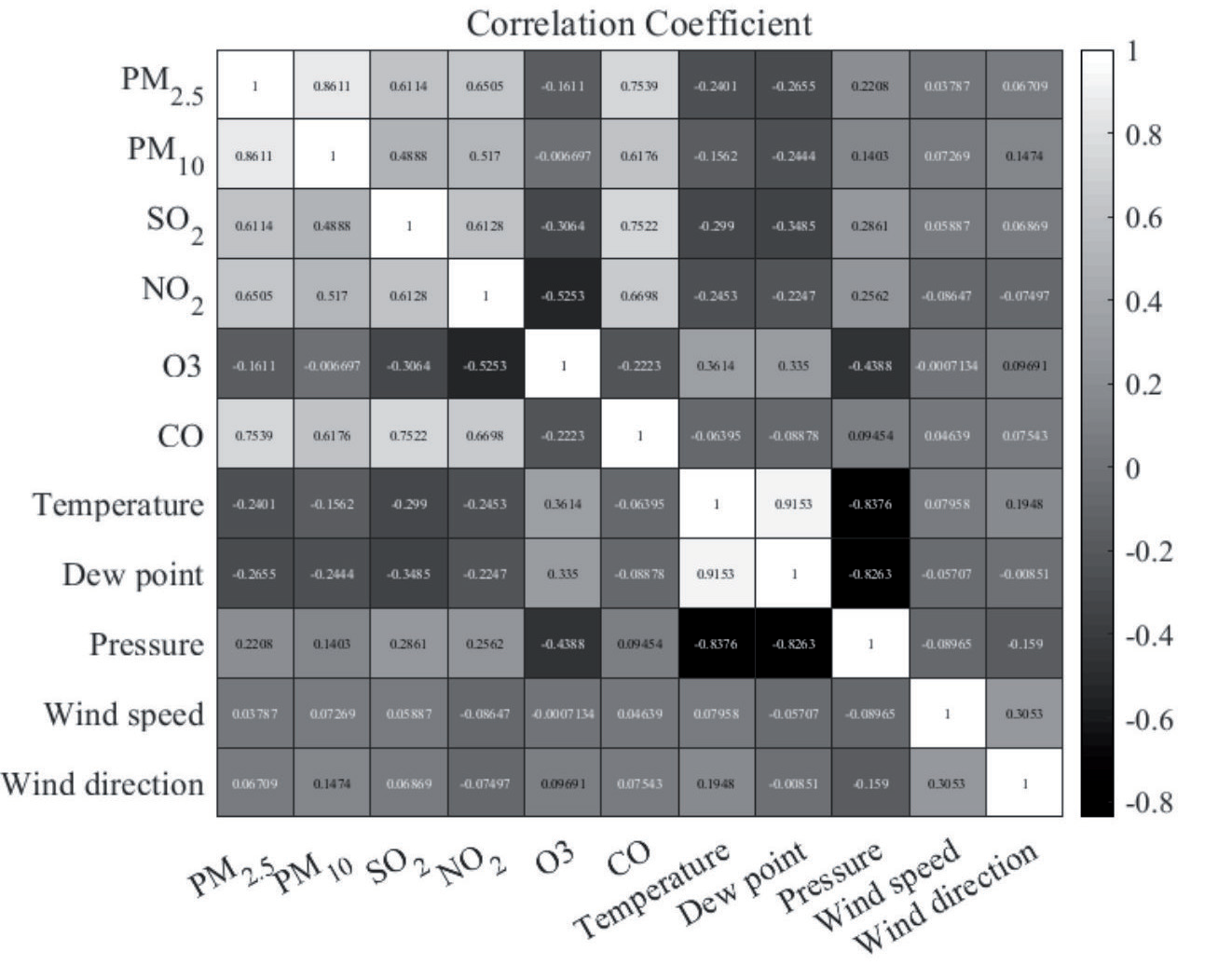
Fig. 3.
PWA model for predicting PM2.5 a) Comparison between observed data and prediction b) fit comparison between observed data and prediction.
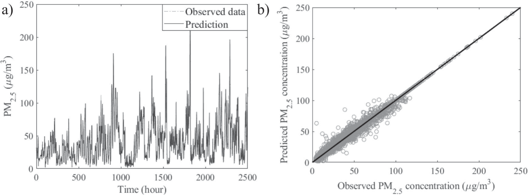
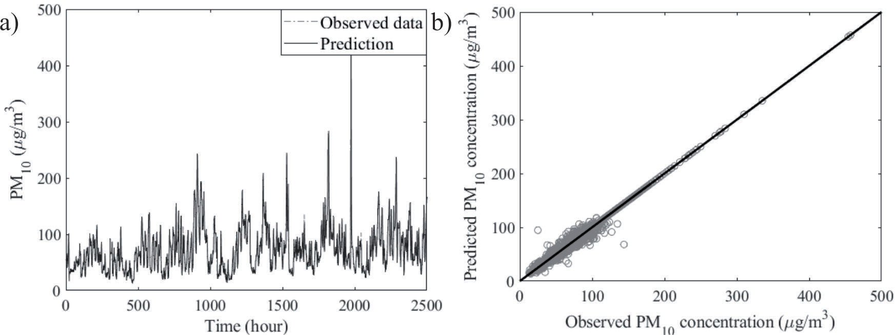
Table 1.
Performance of the PWA model.
| Assessment | Air pollutant | ||||
|---|---|---|---|---|---|
| PM2.5 | PM10 | SO2 | NO2 | CO | |
| MAE | 3.1432 | 2.8859 | 2.5238 | 3.1185 | 0.0770 |
| RMSE | 5.1462 | 5.2701 | 4.2518 | 4.6505 | 0.1211 |
| R | 0.9856 | 0.9914 | 0.9544 | 0.9654 | 0.9708 |
Table 2.
Comparison of different models.
When other air pollution, like PM10, is predicted using the proposed approach, the prediction values generally still match the observed data. Fig. 4 results show that the proposed approach may be effectively used for PM10 prediction with a similar outcome to PM2.5. As all of the pollutants in Table 1 have R values for the prediction over 0.95, the model that was provided can accurately forecast the air pollution.
Comparison with Other Methods
This work compares the proposed PWA model with several baseline techniques, like SVM, MLP, ARIMA, LSTM, and the Bi-LSTM model, to evaluate the effectiveness of the proposed approach. The outcomes of the suggested PWA model are shown in bold. In this study, several models are built using the same data sets, but the input sequences are altered by the structural differences between the models. The proposed model is contrasted with alternative models for PM2.5 prediction in Table 2. Due to the constraints of the model architectures, MLP, ARIMA, and SVM display significantly more significant mistakes, although both LSTM and Bi-LSTM, two deep learning techniques, performed better. Table 2’s MAE, RMSE, and R values show that the model that was proposed for this study performed better in terms of prediction than the other baselines. Additionally, it is better able to depict the features of pollutant concentrations. Overall, the performance of the suggested model was enough for the prompt implementation of additional safety measures using realistic prediction tasks.
Conclusions
The data-driven PWA method was proposed in this work to predict air pollution. Initially, a new clustering-based technique was used to find a data-driven PWA model for air pollution prediction. The widely used BIRCH algorithm was enhanced by the suggested clustering approach, which added a refinement step to handle clusters of any shape. Next, global optimization is used to estimate both the model order and parameters at the same time.
This study employed this approach to forecast Shenyang, China’s air pollution, and it compares the performance of the suggested model to the baseline models. The proposed models for predicting air pollution were compared against several baseline models. The proposed approach, according to the results, might successfully generate models with higher quality that are more suitable for early warning of higher air pollution concentrations and for developing trustworthy management measures for effective environmental protection. The proposed approach may be used in future research to forecast more air contaminants in different regions. The second research would target the enhancement of model quality by taking into account other potential affecting factors.

