

Introduction
Amidst the global march towards industrialization, nations are earnestly committed to economic development, inevitably entailing the extensive utilization of fossil fuels such as oil, coal, and natural gas. This pursuit, however, carries the weighty consequence of substantial CO2 emissions, contributing significantly to the urgent challenge of global warming. Addressing this environmental crisis, the 1997 Kyoto Protocol introduced the groundbreaking concept of “carbon emission trading,” treating carbon dioxide emission rights as tradable commodities. This initiative gave rise to a novel market that intricately intertwines economic interests with ecological considerations.
Acknowledging its substantial contribution to emissions, China embarked on a mission to establish pilot carbon emission rights exchanges in key cities and provinces, including Shenzhen, Beijing, Shanghai, and Hubei, commencing in 2013. A significant milestone was reached on July 16, 2021, with the official launch of the national carbon emission trading market. Positioned as a crucial economic instrument for carbon emission control, carbon trading is poised to propel China towards its ambitious environmental goals of achieving a “carbon peak in 2030” and attaining “carbon neutrality in 2060.”
At the core of China’s strategy for sustainable development lies the dual-carbon strategy, a fundamental national policy. The carbon market represents a pivotal innovation within China’s climate governance framework, signaling a departure from past reliance on administrative directives and financial subsidies towards a market-driven carbon pricing mechanism in response to climate change. The role of the carbon market is indispensable in the nation’s pursuit of carbon peak and carbon neutrality goals. Since the inception of China’s carbon trading pilot market, its prices have undergone notable fluctuations and transformations. As the Chinese carbon market continues to mature, establishing stronger connections with the energy market, stock market, financial market, and other relevant sectors, the application of big data analysis methods assumes paramount significance in unraveling the intricate dynamics of China’s carbon market price fluctuations.
Literature Review
The existing research on the carbon trading market has laid an analytical foundation for us. From the perspective of literature development, the EU carbon market was the earliest and most mature. In terms of the fluctuation characteristics of carbon trading prices, foreign carbon trading markets have been established for a longer time, the trading system is more developed, and the market is more mature. The existing literature mainly focuses on the following aspects: first, the price fluctuation of the carbon spot market; Second, the price fluctuation in the carbon derivatives market; The third is the dynamic relationship between the carbon spot market and the carbon derivatives market. Daskalakis et al. found that carbon storage quotas would have a negative impact on the effectiveness and liquidity of the carbon spot market [1]. Feng Zhenhua and Wei Yiming used the CAPM model to analyze the price risk of the EU carbon market and examined the fluctuation of the EU carbon quota price under different expected returns [2]. Huang Jie found that the yield of carbon futures contracts in the EU has a strong volatility agglomeration through the establishment of GARCH model, and there is a causal relationship between the price of EUA and CER futures, and accordingly put forward relevant suggestions for the establishment of a carbon futures market in China in the future [3]. Gorenflo’s research shows that the EU carbon futures price leads the carbon spot price [4]. Zhang Chen and Liu Yujia extended the research on carbon market spillover effects to the three markets of EU carbon spot, carbon futures and carbon options. The research found that there are significant mean and volatility spillover effects in the three markets, and the carbon derivatives market is the main risk spillover source of EU carbon market [5]. However, since the EU has established a unified carbon market from the beginning, there is no transition stage of regional pilot, so there is no relevant research on the spillover effect of the regional carbon market. Zhang et al. analyzed the scale of international carbon emissions trading and the unfair distribution of benefits under the framework of the Kyoto Protocol based on the equilibrium price of the marginal emission reduction cost and the market price of emission rights, and found that developed countries occupied the leading position in the pricing power of international carbon emissions trading and obtained considerable benefits from it. Then, it is necessary for developing countries to carry out reasonable assessment and long-term planning for carbon emissions trading [6]. Joyeux and Milunovich used the carry-cost model to study the market efficiency of CO2 emissions of EU futures market from June 2005 to December 2007, and found that the estimated model parameters began to approach their theoretical values when approaching smaller samples [7]. Research shows that carbon emissions can be controlled through carbon emissions trading [8], carbon emissions pricing plays a key role in achieving emission reduction goals [9], and the peak value of domestic carbon emissions trading volume and carbon emissions price fluctuations are highly concentrated [10, 11]. In the foreign carbon market, the price fluctuation of the EU carbon quota market has a significant “leverage effect” in both stages [12], and the jump of the EUA spot market shows dynamic time-varying and jump diffusion [13]. According to the trading price data of seven regional carbon markets established in China, the trading price fluctuation of carbon emission rights is mainly characterized by small volume and large price difference [14], volatility spillover effect [15] and nonlinearity [16]. Relevant research also further confirmed that there is a long-term stable relationship between international carbon futures prices and domestic carbon prices, showing an obvious one-way causal relationship [17, 18]. According to the characteristics of carbon market price fluctuations, Wang Jiazhen and others identified five major risks leading to carbon market price fluctuations, including policy risk, liquidity risk, macroeconomic fluctuation risk, risk of participants, and spillover risk. To prevent the risk of carbon market price fluctuations, they put forward risk prevention suggestions to improve the carbon market trading system, improve the financial attributes of the carbon market and prevent other market spillover effects in advance [19]. Fan Liwei et al. proposed the SSA-SVR decomposition integrated prediction framework based on a rolling time window [20]. Li Yao used nonlinear Granger causality test and social network analysis (SNA) to study the correlation between carbon market prices in eight regions of China [21].
Methods
The carbon price shows the characteristics of “rising in fluctuation” or “falling in fluctuation” in the time series, which is the result of the superposition of long-term trend and short-term fluctuation. Therefore, the “surplus” method should be used to study the fluctuation law of carbon price, and two state sequences of long-term trend and short-term fluctuation should be separated from the price. The long-term trend part reveals the endogenous, stable, and predictable change law of carbon emission trading price, while the short-term fluctuation part reveals the seasonal and cyclical change law and can be used for volatility analysis. Based on this, this paper uses the H-P filter method and ARCH model to analyze the fluctuation law and regional characteristics of China’s carbon price.
Census X12 Seasonal Adjustment Method
In the analysis of financial time series, the volatility of a time series is divided into four parts: Trend represents the trend change of the series, Cycle represents the cycle change of the series, Seasonal represents the seasonal change of the series, and Irregular represents the irregular change of the series. In the research of this paper, additive seasonal adjustment is selected to conduct Census X12 seasonal adjustment analysis on domestic carbon price time series data.
If Tt is the trend change item of domestic carbon emission trading price, St is the seasonal change item, Ct is the cyclical change item, It is the irregular change item, and the Census X12 addition model is used, the domestic carbon price can be expressed by the following formula:
Through the Census X12 seasonal adjustment method, the seasonal variation St and irregular variation It are separated from the carbon price Pt, and the sequence trend variation Tt and cyclic variation Ct are included in the remaining long-term trend components of the carbon price time lattice series. For further research, this paper introduces the H-P filter method to separate the long-term trend into the trend variation Tt and cyclic variation Ct.
H-P Filter Model
The H-P filter method was proposed by Hodrick and Prescott in 1980 when they analyzed the post-war economic prosperity of the United States. The H-P filtering method assumes that a time series Yt is composed of two parts: the time series trend component Tt and the time series cyclic variation Ct, the H-P filtering is to separate the trend component Tt from the time series Tt. In general, the trend component T in time series Y is also known as solving the minimum value:
In the formula, λ represents the positive penalty factor of the trend component Tt, c(L) represents the delay operator polynomial, and L is the delay operator of the trend component Tt , where c(L) = (L–1) – (1 – L). Substitute (3) into (2), then in this study, the problem solved by H-P filtering is to solve the minimum value of the following formula:
Then, the optimal value of λ is expressed as:
Therefore, the trend component Tt and cyclic change ct are respectively expressed as:
When the value of λ is λ = Var(ct)/Var(Δ2Tt), the effect of H-P filtering is the best. In the H-P filtering method, the variable λ is called the conversion factor. Experience has shown that the value of λ is very important for the analysis effect of H-P filtering. In the study, if annual series data is selected, the value of λshould be 100; If quarterly series data is selected for research, the value of λ should be 1600; When the study series is monthly data, λ is 14400. In this study, considering the availability of data, the monthly data of domestic carbon emissions trading price is selected, and the value of λ in H-P filter analysis is 14400.
ARCH Models
The autoregressive conditional heteroskedasticity model (ARCH) was first applied in the analysis of stock market price fluctuations. Fama observed in 1965 that the changes of speculative prices and returns have stable and volatile periods, that is, the price fluctuations are clustered. Engle first proposed the ARCH model and its extended model in 1982. This model solves the problem of time-varying variance modeling and is often used to describe the conditional heteroscedasticity and volatility clustering of time series [22]. The ARCH model, originating from observations on stock market behavior, has evolved into a crucial instrument for modeling time-varying variance and explaining volatility clustering in various time series data, contributing significantly to the field of financial econometrics.
In recent years, ARCH models have been increasingly applied to the study of price fluctuations. ARCH model is composed of two equations, and its general expression is as follows:
Formula (8) is the mean value equation, and Rt is the carbon price yield; Rt–1 is the explanatory variable, the lag term of Rt; εt is the stochastic disturbance. Formula (9) is a variance equation, where σt2 represents conditional variance of εt, including constant term a0 and ARCH term ∑t a ε −q=1 t t2 1 ; q is the lagging order. If one coefficient in ARCH term is significantly not equal to 0, it means that the conditional variance of random disturbance term is affected by the previous variance, that is, there is volatility clustering.
Linear GARCH (p, q), ARCH-M model and TARCH model are the extended models of ARCH. The conditional variance of the linear GARCH (p, q) model is not only a linear function of the square of the lag residual, but also a linear function of the lag conditional variance. GARCH model is suitable for describing high-order ARCH processes conveniently when the amount of calculation is small, so it has greater applicability. The expression is as follows:
While the magnitude of
ARCH-M model introduces ht into the mean value equation of ARCH model to measure whether there is high risk and high return. The expression is:
In formula (12): if the coefficient γ is positive, it means that the market supplier will determine the corresponding price according to the risk of price fluctuation, that is, there is a risk reward characteristic of “high risk and high return”. TARCH model is used to analyze the asymmetry of volatility. Its conditional variance expression is:
In formula (13): dt–1 is dummy variable, when εt– 1<0, dt–1 = 1;when εt–1>0, dt–1 = 0. In this model, when φ ≠ 0, the price fluctuation is asymmetric; When φ>0, it indicates that the fluctuation caused by price decline information is greater than that caused by price rise information; When φ<0, it indicates that the fluctuation caused by price rise information is greater than that caused by price decline information.
The ARCH effect holds paramount importance in the realm of carbon markets. Its crucial role lies in unraveling the intricate patterns within price fluctuations. By capturing phenomena like volatility clustering and conditional heteroscedasticity, the ARCH effect enables a nuanced understanding of how carbon prices evolve over time. Volatility clustering reveals the tendency for carbon prices to exhibit periods of similar volatility, offering insights into potential market trends. Meanwhile, recognizing the non-constant variance of price changes is pivotal for anticipating and adapting to shifting market conditions. This comprehensive insight empowers policymakers, investors, and market participants to make informed decisions and develop strategies attuned to the dynamic nature of carbon markets.
Results and Discussion
Data Sources
Since 2005, China has been the world’s largest energy consumer and carbon emitter, and its carbon emissions have also increased year by year. China’s use of market mechanisms to control greenhouse gas emissions began with the clean development mechanism under the Kyoto Protocol. China’s current carbon trading market is still in the early stage of construction. Starting from the CDM project in the Kyoto Protocol, it is divided into three stages: the clean development mechanism stage (about 2002-2011), the pilot trading stage (2011-2020) and the national trading stage (2020-present). The trading varieties of China’s carbon trading market during the pilot period are local quota spot and China certified emission reduction (CER) spot, with local quota as the leading factor. Since 2011, seven carbon trading pilot projects have been launched in Beijing, Tianjin, Shanghai, Chongqing, Guangdong, Hubei, and Shenzhen to explore the establishment of a carbon trading mechanism. Among them, Shenzhen Carbon Emission Rights Exchange is the first carbon emission rights exchange opened in China, and the most active exchange on China’s market. Fig. 1. shows the cumulative turnover and volume of carbon market.
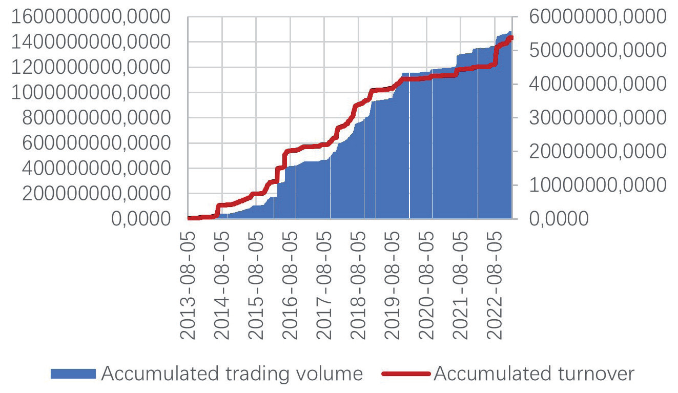
According to the daily closing price data of the eight carbon trading pilots from 2013 to 2023, the carbon prices of the eight carbon markets showed a downward trend in general from 2014 to 2023. From 2016, the average value of the transaction prices of the eight carbon markets gradually stabilized at about 25 yuan/ton. Although the price fluctuation of carbon emissions in various markets presents different characteristics of sustainability and asymmetry, it has convergence in the range and trend of change. Based on the fact that Shenzhen Carbon Emission Exchange is the earliest place for carbon emission trading in China, which is convenient to study the rules and characteristics of carbon price fluctuations, and considering the consistency of the time span of each data, this paper selects the monthly price of Shenzhen Carbon Emission Exchange from August 2013 to February 2023 as the representative of the domestic carbon emission trading price, with the unit of yuan/ton of carbon dioxide, and a total of 116 monthly trading data. The price data comes from the Shenzhen Carbon Emission Trading Exchange and Wind database. The Shenzhen carbon emission trading price is expressed as Carbon.
Periodic and Trend Analysis
Trend Analysis
The Census12 seasonal adjustment method is selected by Eviews12.0 software to analyze the carbon emission trading price series from 2013 to 2023. The Shenzhen carbon price SP from 2013 to 2018 is decomposed into seasonal variation component S, irregular variation component I and long-term variation component TC of the price series. The formula is expressed as follows:
In the formula, SP represents the trading price of carbon emission rights in Shenzhen; TC represents long-term change; S represents seasonal variation; I represent for irregular change; T and C represent trend and cycle change.
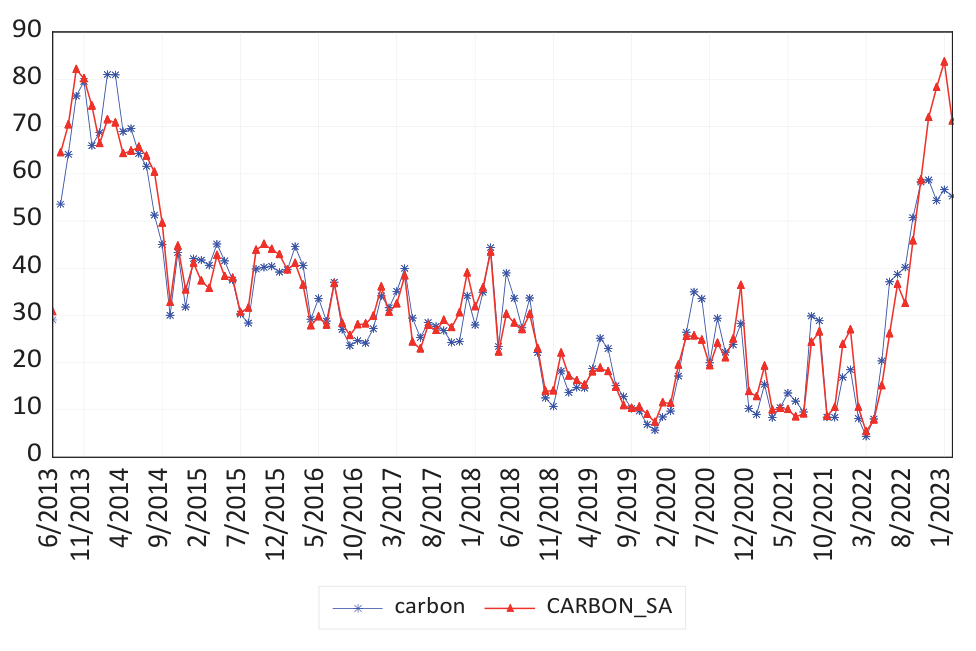
It can be seen from Fig. 2. that the carbon price and the seasonally adjusted price of Shenzhen carbon emission trading market show a fluctuating trend. The blue line in the figure represents the Shenzhen carbon price, and the red line indicates the fluctuation trend of carbon price after seasonal adjustment. It can be concluded that the trading price of carbon emission rights in Shenzhen has shown a downward trend since 2013. With the change of trading time, the price fluctuation has shown obvious cyclical changes. The trading price of carbon emission rights in Shenzhen reached the historical peak of 81.09 yuan/ton of carbon dioxide in February 2014, and reached the historical minimum of 23.49 yuan/ton of carbon dioxide in September 2016. In more than two years, the trading price of carbon emission rights in Shenzhen decreased by 57.6 yuan, 2.36 times of the lowest price.
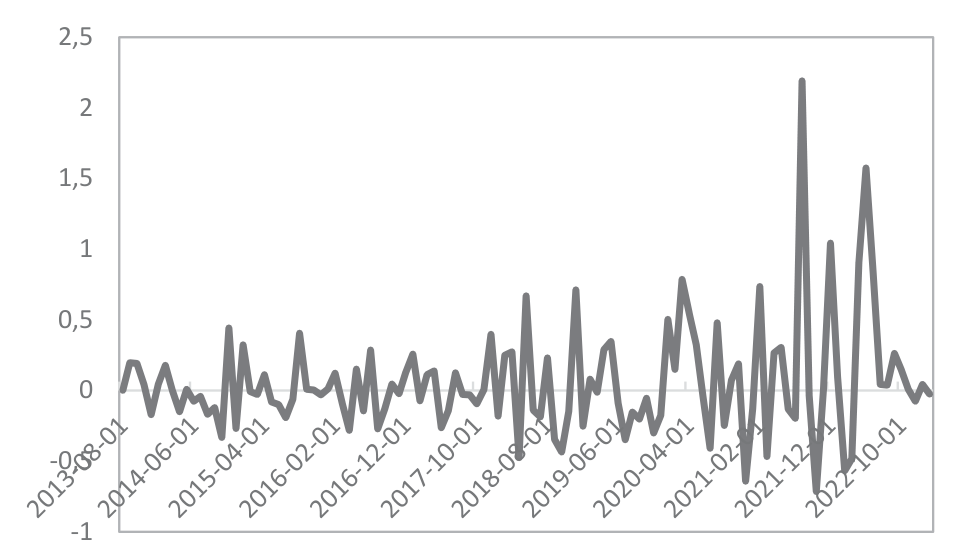
It can be seen from the month-on-month growth trend in Fig. 3. that the month-on-month growth rate of carbon emission trading price in Shenzhen reached the highest in history in September 2015, with a month-on-month growth rate of 0.4%, and reached the lowest decline in history in October 2014, with a decline of 0.51%.
Periodic Analysis
The variable carbon represents the long-term change trend of carbon price from 2013 to 2023. To study it more accurately, this paper uses the H-P filter method to decompose the sequence and separate the trend change trend and cycle change of Shenzhen carbon emission trading price. The decomposition results are shown in Fig. 4. It can be seen from Fig. 4. that the carbon price showed a steady downward trend from August 2013 to January 2023, showing a relatively obvious cyclical change rule.
Fig. 2.
The carbon price and the seasonally adjusted price of Shenzhen carbon emission trading market.
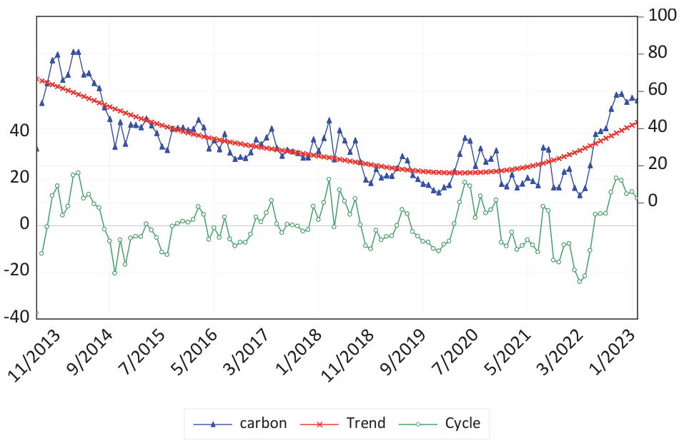
In this paper, the H-P filter method is selected in the study, and the whole carbon price series is divided into five complete cycles according to the trough - trough. Table 1. describes the cycle characteristics of carbon price fluctuation from 2013 to 2023. China’s carbon price fluctuated sharply in 2013 and 2020, with significant price fluctuations. However, from 2015 to 2017 and from 2011 to 2020, China’s carbon price fluctuated relatively gently, with a small price increase. The duration of the violent fluctuation period was shorter, and the duration of the stable fluctuation period was longer.
Seasonal and Irregular Variation Characteristics
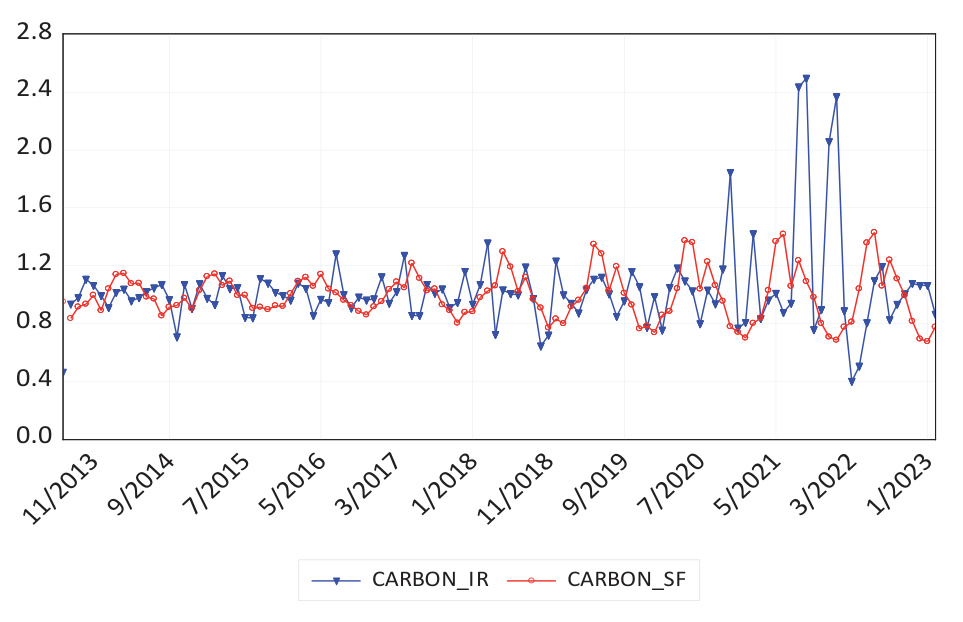
Fig. 5. describes the seasonal and irregular variation factors separated from the monthly carbon price data of China from 2013 to 2023. It can be seen from Fig. 5. that the seasonal variation of China’s carbon price is a sine function, with obvious regularity. Every year, there is a cyclical change in the rise and fall, and the range of rise and fall is balanced. The range of price rise and fall in each cycle is around 0.8-2.5 yuan/ton of carbon dioxide equivalent. Due to the influence of many factors, the irregular change of carbon price in China shows the characteristics of random fluctuation, but the overall fluctuation tends to moderate. From 2014, the change range exceeded 1.2 yuan/ton of carbon dioxide equivalent, to less than 0.9 yuan/ton of carbon dioxide equivalent in 2016.
From the research results, we can see that since 2013, China’s carbon price has shown different trends. In 2013, the overall carbon price is high, between 60-80 yuan/ton of carbon dioxide equivalent, and the price is at the peak of the previous 10 years. However, in 2014, the carbon price fell sharply from 80 yuan/ton of carbon dioxide equivalent at the beginning of the year to 30 yuan/ton of carbon dioxide equivalent at the end of the year. In the next four years, from 2015 to 2018, the carbon price changes in a highly similar pattern, rising slightly at the beginning of each year, reaching the lowest point in July in the second half of the year, and then beginning to remain unchanged, with no obvious change. Since 2020, the carbon price has increased significantly.
Table 1.
Carbon price cycle division.
Table 3.
Regression results of ARCH model.
ARCH Effect Analysis
Test for Data Stationary
The ARCH effect test requires that the price data must be stable. Therefore, it is necessary to carry out the ADF test on the carbon price yield series. See Table 2. for details. The price yield series has passed the stability test at the significance level of 1%. Therefore, it is considered that the carbon price and yield series are stationary and can be tested by ARCH effect.
Regression Results of ARCH Model
ARCH regression analysis was used on the carbon price yield series, and the results are shown in Table 3. It can be seen from Table 3. that the ARCH coefficient “a” has passed the stationarity test, and α1 is significant at the 1% level, indicating that the carbon price fluctuation has significant clustering. The estimated value of γ in the ARCH-M model is -0.526, but it is not significant, which does not indicate that the carbon market has the characteristics of high risk and high return. In the TARCH estimation results, the estimated value of φ is less than zero and significant, indicating that the carbon price fluctuation in China has significant asymmetry, that is, there is a feature that the fluctuation caused by price rise information is greater than that caused by price decline information.
Conclusions
This paper selects the monthly data of carbon emission trading prices in Shenzhen from August 2013 to February 2023 to represent the national carbon market prices, and uses the H-P filter method and ARCH cluster model to study the fluctuation law and cycle characteristics of carbon emission trading prices in China. The research results show that from 2013 to 2023, China’s carbon emission trading price had a significant downward trend and cyclical characteristics.
(1) In the short term, the seasonal cycle of China’s carbon price is obvious. Between 2013 and 2020, China’s carbon price fluctuated sharply. From 2015 to 2017, the carbon price fluctuated relatively gently, and from 2011 to 2020, the price increase was not very large as well. The duration of the violent fluctuation period was shorter, and the duration of the stable fluctuation period was longer. In the four complete cycles, the time range of each cycle is 10-26 months, and the peak and valley values show a downward trend of varying degrees. The peak and valley values change from positive to negative, and the cycle types show a steep downward trend. In 2013, Shenzhen took the lead in launching the first carbon emission trading market, and the domestic carbon emission trading market was relatively small, so the overall carbon price in 2013 was high. After 2014, other pilot projects began to start in succession, and the carbon price in Shenzhen was affected and began to fall. From June to July of each year, the temperature is higher, and the carbon price is lower, which means that the higher temperature reduces the energy demand, thus reducing the carbon dioxide emissions, and reducing the carbon price.
(2) In the long run, the carbon price changes periodically every 20 months or so, with the fluctuation range of 2-7 yuan/ton of carbon dioxide equivalent. At the same time, the carbon emission trading prices in other regions in China will also fluctuate to different degrees. The cyclical fluctuation amplitude of carbon price is relatively intense. Considering the dynamic change angle, China’s carbon price fluctuation shows a trend of “short cycle, small amplitude”, and the fluctuation characteristics show a shorter cycle and smaller amplitude. From the specific research results, the fluctuation height of the four complete cycles has declined and flattened, the breadth of price fluctuation has increased slightly, and the contraction length in the four complete cycles is not less than the expansion length. These characteristics indicate that China’s prices have a downward trend in the four cycles studied, which is consistent with the overall trend fluctuation characteristics.
China is a major carbon emitter. According to statistics, the world’s total carbon dioxide emissions from energy consumption in 2012 were 3231028712 million tons, and China’s carbon dioxide emissions from energy consumption were 8106.43005, accounting for about 25.1%. In 2015, domestic carbon emissions accounted for 1/3 of the total global carbon emissions. Although the Kyoto Protocol does not mandate emission reduction, to ensure the sustainable development of the global economy, China has also taken the initiative to assume the responsibility for emission reduction. The fluctuation of the domestic carbon emission trading price and regional characteristics will also have an increasing impact on China’s future energy and economic development.
Based on the findings of the study, here are some policy recommendations for the carbon market in China:
Strengthen Carbon Market Oversight and Transparency. Given the cyclical fluctuations and downward trend observed in carbon prices, it is recommended that the government strengthens oversight and transparency in the carbon market. By implementing a more rigorous regulatory framework, including more frequent market reviews and reporting requirements, the government can identify and address potential market risks in a timely manner. Enhancing market transparency can also boost investor confidence, attract more participants, and foster the healthy development of the carbon market.
Encourage Carbon Price Stability. To mitigate the trend of carbon price volatility, the government may consider measures to promote price stability. This could involve introducing market incentive mechanisms, such as establishing a carbon price floor or implementing price intervention mechanisms to prevent excessive price fluctuations. Such policies would help attract more investors and steer the carbon market towards a more sustainable and robust direction.
Enhance International Cooperation and Carbon Market Linkages. Given China’s status as a major global carbon emitter, the government could actively seek cooperation and linkages with carbon markets in other countries and regions. Establishing international mechanisms for collaboration in carbon markets can contribute to greater price stability and facilitate the achievement of global carbon reduction goals. This international cooperation can also help mitigate the impact of domestic carbon market fluctuations on the Chinese economy and improve the overall efficiency of global carbon markets.
These policy recommendations aim to provide a more stable and sustainable development trajectory for the carbon market in China, enabling it to play a leading role in global carbon reduction efforts.