

Introduction
The global oceanographic dynamics of the Pacific Ocean significantly impact the Makassar Strait, making it a distinctive maritime passage in Indonesian waters. The Indonesian Throughflow (ITF) channels water from the Pacific to the Indian Oceans, as noted by [1]. The ITF’s movement affects climatic variability across various time scales, from intra-seasonal and seasonal to inter-annual [2]. ITF fluctuations are strongly associated with ocean-atmosphere dynamics in the equatorial area during an intra-seasonal period. As a direct effect of climate change, the sea surface temperature has increased, and the ocean has warmed over the past few decades, causing changes in global precipitation and ocean circulation patterns, a decrease in sea ice extent, and an increase in sea level [3].
Ocean warming impacts the distribution of marine species, causing fish populations to shift to deeper water or higher latitudes when ocean temperatures rise [4]. Experts estimate an 89% decline in global fishery income. Countries will experience a decrease in maximum potential income in 2050 in the high-emissions scenario (RCP8.5) in line with climate change, a reduction in fish numbers in the tropics, and an increase in fish readings in temperate areas [5]. One of the primary consequences of climate change is an increase in sea surface temperature (SST), potentially impacting tuna fisheries [6].
The Eastern Little Tuna (ELT), a small pelagic fish, serves as one of Indonesia’s main export commodities. Information about tuna fishing areas is crucial for the success of fishing operations [7]. Sea surface temperature (SST) is an important factor for the life of organisms in the sea because it can influence the metabolic activities of species [8]. Various indicators, including sea surface temperature, can predict the movement and distribution patterns of ELT, a small pelagic fish species [7]. Numerous research studies, like those by [9, 10, 11, 12], indicate that sea surface temperature (SST) is a constraining factor affecting the distribution, abundance, and physiology of tuna, while also indirectly impacting migration patterns. Sea surface temperature significantly impacts spawning, feeding behavior, and salinity levels in fish, especially tuna [13], and influences predator-prey interactions [14].
A spatial information technique based on oceanic factors can be used to get information on fishing areas [15]. According to [16], oceanographic factors such as SST impact fish catches in seas. Understanding the evolving risks and forces causing change in marine communities and the region most likely impacted is essential for sustainable exploitation and management of ecosystems [17, 18]. The objectives of this study are to identify the habitat preferences of eastern little tuna and to ascertain how the shift in the Potential Fishing Zone (PFZ) is affected by increasing SST conditions and the catch of eastern little tuna.
Comprehending the correlation between SST and ELT is essential for sustainable fisheries management and enhancing fishing strategies. Efficient monitoring of SST patterns enables stakeholders to anticipate ELT occurrences, improve capture efficiency, and reduce the likelihood of unsuccessful fishing expeditions. Given the escalating worries regarding climate unpredictability, evaluating the direct impact of sea surface temperature on ELT fisheries is crucial for protecting the livelihoods of coastal communities and maintaining small-scale fishermen’s socioeconomic conditions.
Materials and Methods
Research Area
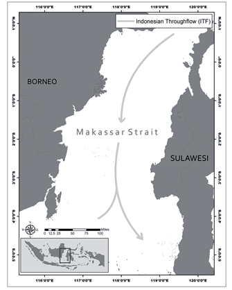
The research area was located between 1°N – 5°S and 115 – 121°E in the Makassar Strait region. According to Fisheries Management Area (FMA) 713, the area was chosen based on oceanic dynamics and the Makassar Strait’s capacity for fishery capture (Fig. 1). The Makassar Strait is considered an ecologically productive location for small-scale tuna fishing in the eastern region. Moreover, the Indonesian Throughflow (ITF) recognizes the research field as one of its paths.
The pressure gradient between the Pacific and Indian Oceans drives the ITF. The Indonesian Sea’s canals and basins allow the Pacific seas to flow into the Indian Ocean. The flow starts in the Strait of Lombok, proceeds via the Strait of Makassar, flows across the Flores Sea, and ends in the Banda Sea. According to [19], the ITF affects the temperature and freshwater reserves in the Pacific and Indian Oceans.
Data
Fishery Data
We processed data spanning six years (2015–2020) to determine the regional and temporal distribution of fish and oceanographic characteristics. Fish datasets are obtained from the logbook of the Ministry of Maritime Affairs and Fisheries, including data on fishing activities, coordinates, fish weight, and fishing gear, processed into CPUE and fishing location. CPUE is computed using the following equation:
Where:
CPUE = catch per fishing effort (kg/trip)
Catch = catch in year t (kg)
Effort = fishing effort in year t (trip)
Sea Surface Temperature Data
SST data is retrieved from the MODIS-AQUA satellite, where it is visualized, and functions are applied to extract oceanographic parameter values. SST data were downloaded from https://oceancolor.gsfc.nasa.gov/ with a 4 km spatial resolution. It provides binary data at level 3, known as Standard Mapped Image (SMI). The study employed monthly temporal resolution data from January 2015 to December 2020. The data collection underwent additional processing in ArcGIS version 10.8 to obtain picture data across the study area.
Maximum Entropy (MaxEnt) and Wavelet Analysis
The maximum entropy (MaxEnt) machine-learning approach commonly combines species occurrence and environmental parameters to determine species distribution [20]. The maximum entropy (MaxEnt) model analyzed the environmental data on ELT presence spots, producing a probability distribution indicative of the chance of ELT existence according to the chosen environmental variable [21, 22]. The model is constructed utilizing default settings, comprising 80% training data and 20% test data. Model validation employing the subsample approach evaluates model performance by partitioning the dataset into multiple subsets. The original datasets were subsampled, resulting in surviving records that exhibited geographical bias [23].
The ELT catch and SST data were subjected to the continuous wavelet transform (CWT) analysis. The temporal distribution of ocean variability from 2015 to 2020 was obtained using the wavelet transform technique. By breaking down dominating signals into several time scales and examining how these signals alter over time, wavelet analysis conducts a time-frequency analysis of these signals. The color bars, representing various wavelet amplitudes, display high energy dispersion in red and low values in blue. According to [24], the thin black line indicates the cone of influence (COI), while the solid black line signifies the 95% confidence level.
Analysis of SST Preferences for ELT by Histogram & MaxEnt
To identify possible ELT habitats, we investigated the relationship between ELT catch and SST data. We used a histogram analysis of the SST data, which correlated with higher CPUE values, to estimate the SST preferences of the ELT. Moreover, these particular SST preference ranges served as thresholds for choosing and forecasting possible habitats (fishing grounds) for the ELT. To evaluate the effects of climate change on potential ELT habitats, we utilized projected SST increases from global climate models based on scenarios provided by the Intergovernmental Panel on Climate Change (IPCC). Furthermore, the MaxEnt model correlates oceanographic variables, often termed predictive variables in this context, with fishing (a response variable). Beyond the habitat suitability index (HSI), the MaxEnt model generates a response curve that shows the range of SSTs suitable for the ELT.
Results and Discussion
Temporal and Spatial Variability of Eastern Little Tuna
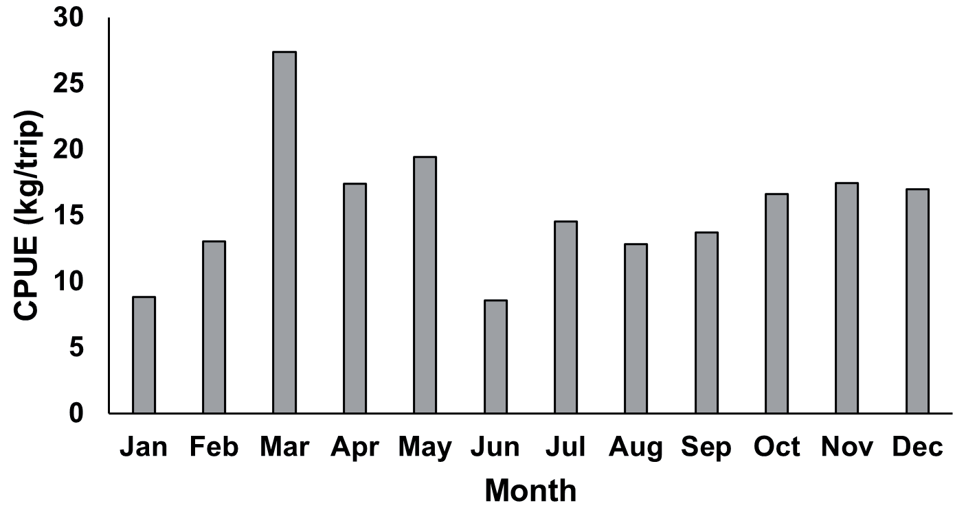
To analyze the fluctuations in the ELT catch rates, we computed the monthly mean climatology of CPUE from 2015 to 2020. Fig. 2 presents a distinct seasonal pattern in the average monthly CPUE values. The monthly mean CPUE of ELT in the Makassar Strait ranges from 10 to 30 kg/trip.
Catch per unit effort (CPUE), a common indicator of fish resource quantity, reflects the efficiency of fishing gear in fish harvesting [25]. The CPUE analysis of ELT, which derives from the aggregate CPUE, establishes the utilization rate and species abundance in waters. March recorded the highest average CPUE, reaching 30 kg/trip, while June recorded the lowest, at 10 kg/trip.
After classifying this ELT catch data into seasonal catches, CPUE is computed by dividing the catch by the total number of trips made each season (Fig. 3). The transitional season I (TS 1) period recorded the highest capture, averaging 21.40 kg/trip, based on the average CPUE value per season. The transitional season (TS 2) recorded the second-highest catch, with an average CPUE of 15.94 kg/trip. During the northwest (NW) and southeast (SE) seasons, the average CPUE is 11.97 kg/ trip and 12.96 kg/trip, respectively. To better understand the SST conditions at the time of the highest ELT catch, we overlaid the SST spatial data on the fishing locations during transitional season 1 (March–April–May 2017) (Fig. 4).
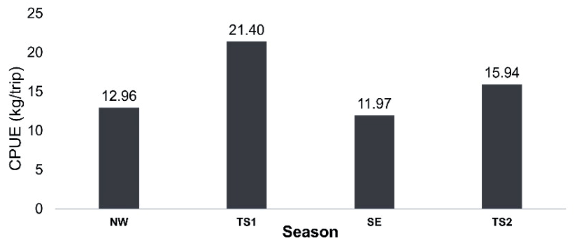
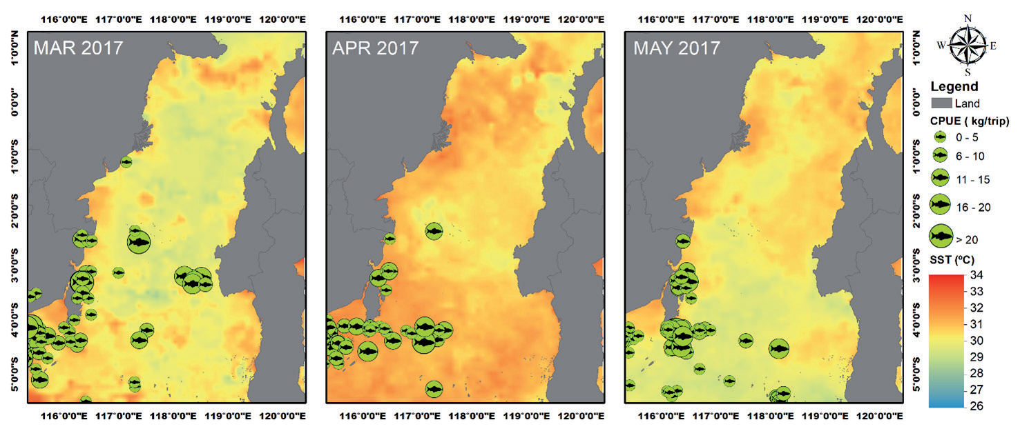
Fig. 5.
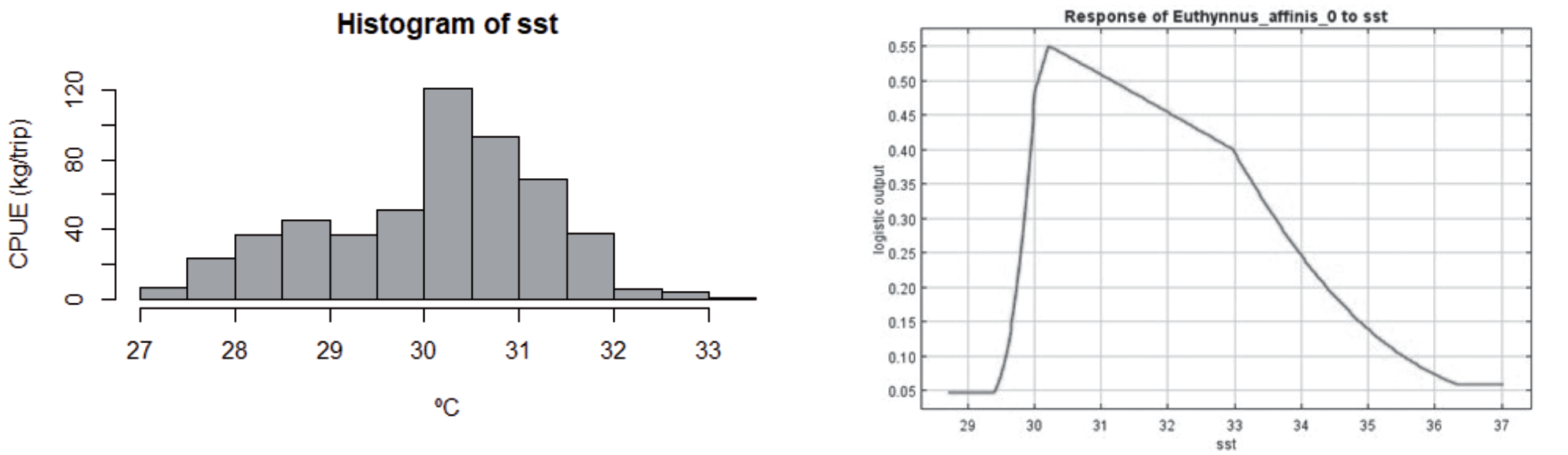
Preferred SST for ELT based on a). histogram, the x-axis shows the SST categories, the y-axis shows the CPUE frequency within the SST range, and b). The response curve of SST is based on the MaxEnt model analysis; the x-axis represents the SST range, and the y-axis represents the predicted habitat suitability of ELT species.
The overlay of SST distribution maps with ELT locations indicates the distribution of the ELT in the center and western waters of the Makassar Strait, near the coast of Kalimantan Island. The ELT is found primarily in the regions of 1°S - 5°S and 115°E - 118°E. The average CPUE ranged from 13.4 kg/trip to 38 kg/ trip in 2017, with numerous fishing spots throughout the Makassar Strait, especially during the TS 1 (March-May), when the SST was between 29°C and 32°C. Various biological and environmental factors have been linked to the behavior and survival of Eastern Little Tuna [26]. According to [27], a body of water with a high SST variability is suitable for fishing activities, as it impacts the migration, spawning, and feeding patterns of fish.
SST Preferences of ELT
An analysis of the histogram of SST data, which showed a correlation with higher CPUE values, was utilized to determine the monthly SST preferences of the ELT (Fig. 5a). These preferences were subsequently confirmed through the MaxEnt model. The identified SST preference ranges were then used as thresholds for selecting and predicting the ELT’s preferred habitats. The Maximum Entropy (MaxEnt) model is utilized to determine the association between the catch rates of ELT and SST. The MaxEnt model generates the response curve, which shows the explanatory variable (SST) values that positively affect the response variable. The response curve’s x-axis shows the explanatory variable’s value, and the y-axis shows the ELT’s probability (Fig. 5b). The positive influence determined ELT’s explanatory variable range. According to the histogram analysis and response curve (Fig. 5), the ideal SST for ELT presence is 30–31ºC.
Fig. 6.
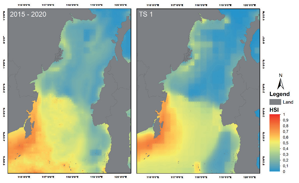
Habitat Suitability Index (HSI) map for ELT based on the MaxEnt model for all seasons (left) and the transitional season 1 (TS1) (right). The color scale illustrates HSI predictions, with blue color representing the lowest (0) and red representing the highest HSI (1).
The histogram analysis findings illustrate the relationship between sea surface temperature and ELT CPUE values from 2015 to 2020. The histogram analysis determined the optimal SST value in the tuna fishing zone by assessing the correlation between maximum CPUE and various SST values. The histogram indicates that SST values between 30 and 30.5ºC yield the highest CPUE (100 kg/trip). These findings align with previous research by [28], which indicated that tuna favor a sea surface temperature between 30 and 30.5ºC. Additional research by [29] found prospective skipjack tuna hotspots in the Makassar Strait (FMA-713), revealing that the optimal sea surface temperature ranged from 29.5 to 31ºC.
The Maxent model outputs estimate ELT habitat in a certain range and offer a spatial map showing ELT capture habitat suitability index (HSI). The Makassar Strait’s expected fishing zone map for the season, including transitional season 1, will depend on the result. The map shows HSI projections in blue for low and red for high (Fig. 6).
Analyzing the prediction map of ELT from 2015 – 2020 and Transitional Season (TS) 1, the habitat suitability index map indicates that the southern Makassar Strait is a suitable area for the occurrence of ELT. Despite the lack of significant variation, the HSI value obtained for the entire year was between 0.5 and 0.9, corresponding to coordinates of 2–5ºS and 116– 118ºE. In the meantime, the HSI value during the TS 1 period indicated that the region suited for ELT habitat was identified between coordinates of 2–5ºS and 116– 117ºE. Compared with the 2015–2020 HSI results, the HSI area is narrower at TS 1.
Wavelet Spectrum Analysis of ELT and SST
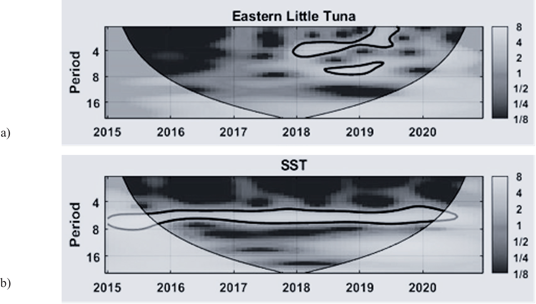
Wavelet analysis (Continuous Wavelet Transform, or CWT) determines the dominant period associated with the amplitude and time phase series. Fig. 7 displays the energy density spectrum pattern for the oceanographic parameters with 95% confidence intervals. On the graph, the y-axis denotes cycle frequency (month), and the x-axis stands for time (year). Wavelet analysis validates the predominant indicators of ELT and SST.
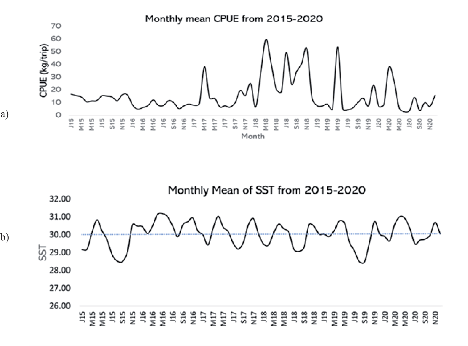
The monthly mean CPUE from 2015–2020 indicates that the ELT catches experienced strong interseasonal signals (6-8 months) from the middle of 2018 to the middle of 2019, as well as intra-seasonal (1-5 months) signals from January 2018 to June 2019. The ELT catches had a significant increment during March 2017 and 2018 (TS 1), September-November 2018 (TS 2), May 2019 (TS 1), and March-April 2020 (TS 1). For the oceanographic parameter, SST has a strong interseasonal (6–8 months) signal along the period of observation. The monthly average time series for 2015–2020 in Fig. 8 clarifies interseasonal variability for ELT and SST.
Based on the temporal variation of CPUE data for 2015 - 2020, there was an increase in catch results in 2018 - 2019. Then, the catch decreased again in 2020. In the meantime, there is a strong intra-seasonal pattern in the average SST, which varies in value every year. The spatial data indicated a tendency toward a warmer average SST distribution from January to May and from October to December. Temperatures in the Makassar Strait are generally warm throughout the year, according to [30], who also noted that there are minimal seasonal fluctuations in SST.
Fig. 7.
Wavelet spectrum analysis of a) the CPUE values for ELT, and b) sea surface temperature (SST) during the years 2015-2020.
Potential Impacts of a 1°C and 2°C Increase in SST on the Habitat Preferences of ELT
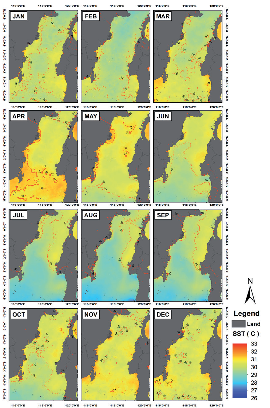
Satellite imagery revealed fluctuations in the SST across various locations in the Makassar Strait, as observed in the average SST data from January 2015 to December 2020 (Fig. 8).
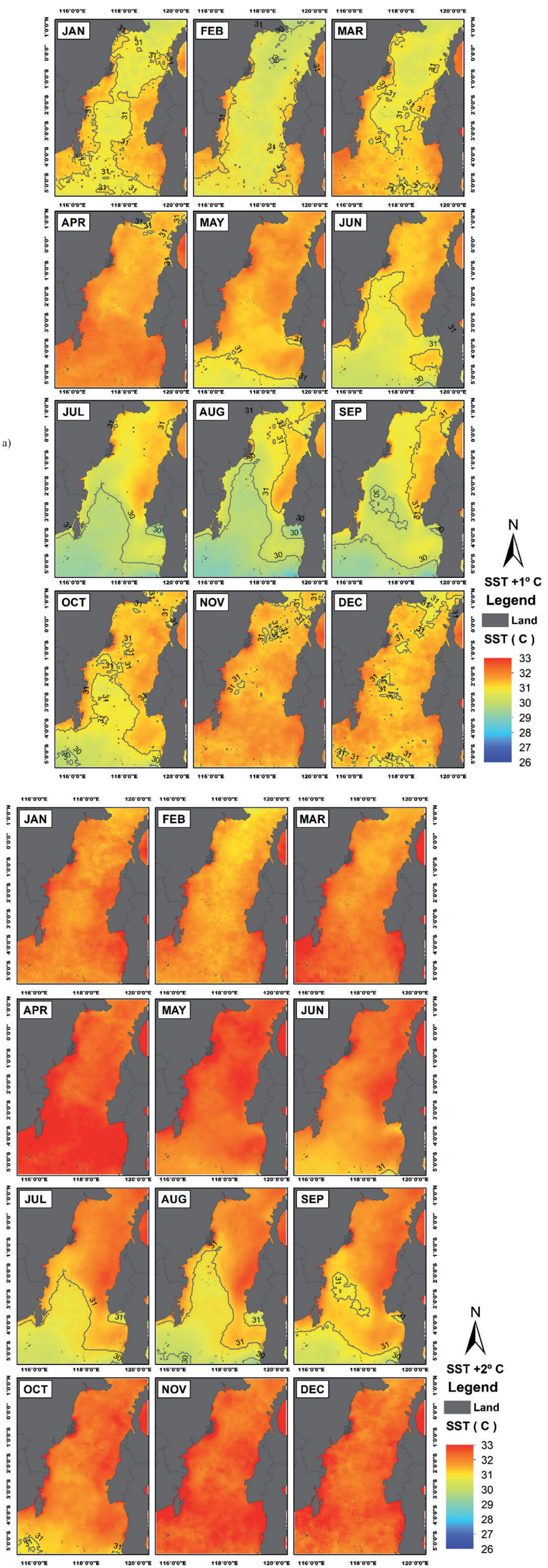
The ideal temperature (30-31ºC) for ELT exists year-round, influenced by seasons, as indicated on the 2015- 2020 SST average distribution map. ELT preferences (30-31 ºC) and average SST in Makassar Strait between 2015 and 2020 suggest ELT is more likely in TS 1 and TS 2 till the NW monsoon. Meteorological factors (rainfall, evaporation, air humidity, air temperature, wind speed, and solar radiation intensity) and oceanic processes (currents, advance, and upwelling) generally impact the SST fluctuation in the Makassar Strait [31]. The change in fishing grounds due to rising temperatures is illustrated in Figs 9 and 10. The contour line of 30-31ºC illustrates the ideal SST for ELT catch.
Fig. 10 depicts the clear boundary line of potential habitats for ELT, influenced by SST increases of 1 and 2ºC. In the early part of the year (January to March), potential habitats with a 1ºC SST increase were primarily located in the central and coastal regions of the Makassar Strait. By April, the preferred habitats of ELT vanish, followed by a southward shift in May. From June to December, the potential habitat boundaries stretched from 4ºS in June to 1ºS in December, under a 1ºC SST rise scenario. A northward shift was observed from July through December.
With a 2ºC increase in SST, the potential habitat preferences of ELT were no longer evident, except during July, August, and September (1-5ºS). SSTs exceeding 31 degrees became prevalent in the Makassar Strait. Furthermore, a 2°C increase in the average SST reduced the fishing season from 6 months to 3 months, with only July through September providing the ideal temperature for the existence of ELT. Due to its impact on the suitability of thermal habitats, temperature appears to be one of the most significant geographical drivers of changes in abundance in marine communities [32].
Discussion
Oceanic and climatic fluctuations affect fish dispersal patterns, not chance. Oceanographic factors like SST may limit fish dispersal and survival [33, 34]. Due to regional and global climate change, oceanographic factors change affect fish distribution and abundance [35, 36]. Climate affects environmental variability and ELT dispersion [33]. SST affects pelagic fish migration, including tuna; hence, climate change affects tuna fisheries [37, 38]. Because the environment strongly affects tuna physiology and behavior, these environmental alterations caused a complicated response [39]. Similar findings showed that SST increase decrease the appropriate habitat for pelagic fish [40].
Tuna spawning and growth have previously been demonstrated to be significantly impacted by sea temperature [41, 42]. Tuna populations may disperse as their preferred temperature ranges change, disturbing their regular mating and feeding grounds. Variations in the amount and distribution of phytoplankton and zooplankton, which are essential tuna prey, can be caused by changes in ocean currents and nutrient distribution [43]. According to earlier studies for other tuna species, warming ocean temperatures may make some habitats more suitable for skipjack tuna [44]. Still, for yellowfin tuna [45], rising temperatures may have a negative impact on the heart function of spawning adults and the survival of eggs and larvae. Fishing activities and, in turn, the efficacy of fisheries management strategies may be impacted by these shifts in the spatial distribution of fish stocks and the composition of fisheries resources [46].
At large regional scales, temperature variations are generally correlated with changes in significant biogeographic patterns, particularly abundance, due to their impact on thermal habitat suitability. Numerous other direct and indirect effects of climate change, such as changing species interactions, including competition and prey availability, hypoxia, ocean acidification, and altered weather patterns, can also have an impact on abundance [47, 48]. Understanding the oceanic factors in a specific location allows one to estimate the existence of fish schools, which can then be used to inform fishing intentions [49, 50].
Tuna populations may shift when their preferred temperature ranges change, potentially disrupting their typical breeding and feeding sites [51]. Fish populations are migrating to higher latitudes or deeper seas due to ocean warming. The geographical redistribution of fish can rapidly alter marine ecosystems [52]. Furthermore, [53] states that changes related to physiological characteristics will affect the predicted distribution of tuna. For example, a decrease in oxygen concentration will hinder the vertical habitat of tuna in the water column.
Research by [54] on the T. albacares species (yellowfin tuna) in Aceh waters indicated that sea surface temperature (SST) is the primary factor affecting the distribution and presence of possible fishing zones. Additional research by [55] in the South Pacific Ocean indicates that the northern boundary of the albacore’s optimal habitat is anticipated to migrate southward as a result of increasing temperatures attributed to climate change. Another study by [56] found that mackerel catch correlates with variations in SST. Mackerel production will rise with an increase in temperature, whilst a decrease in SST will lead to a reduction in catch.
Most organisms’ physiology, which defines their limited temperature ranges, thermal sensitivity, and biological functions like metabolism, growth, and reproduction, determine their vulnerability to warming [57, 58]. Ocean warming will directly affect how fish stocks are managed and assessed and fishing communities are more likely to be affected by changes in fisheries production [59]. Research conducted by [60] revealed a decrease in skipjack tuna catch as SST increased due to the shift in tuna distribution.
Climate change will impact the fisheries sector in three distinct ways. Initially, climate change alters the physical and chemical conditions, including elevated water temperature. Secondly, climate change influences the ecological conditions of the ocean, including the prevalence of illnesses and alterations in species distribution and abundance. Third, it affects socioeconomic conditions, including disrupted fishing activity and diminished fishing productivity [61]. Due to their high vulnerability to economic, health, and environmental risks and shocks, small-scale fishers are considered the most vulnerable socioeconomic group [62]. Small-scale fishers are significantly impacted by climate change, as their social and economic livelihoods rely on weather stability [63]. Elevated water temperatures, unforeseen precipitation, and heightened winds have posed threats of unpredictability and risk in capture fishing, thereby diminishing fish catchability and revenue [64].
This study demonstrated that SST greatly influences the habitat preferences of ELT. The rising ELT catch predominantly takes place in areas with SST between 30-31ºC. The habitat preferences of ELT seemed to diminish under scenarios of rising sea surface temperatures by 1ºC and 2ºC. Moreover, our findings indicated that rising sea surface temperatures from ocean warming can lead to a modification in the fishing season and diminish its duration from six months to three months.
Conclusions
The study found that the transitional season I (TS 1) period saw the highest capture of 21.40 kg/trip when the sea surface temperature (SST) was between 29°C and 32°C. The optimal SST for ELT presence is 30–31ºC. Potential habitats for ELT were primarily in the central and coastal regions of the Makassar Strait. A 1ºC SST increase led to a southward shift in habitat boundaries and a northward shift from July through December. A 2°C increase reduced the fishing season from 6 months to 3 months.