

Introduction
China is one of the countries with the largest energy consumption and carbon dioxide emissions in the world. Fossil energy constitutes over 80% of its overall energy consumption structure [1]. The sixth assessment report of the Intergovernmental Panel on Climate Change (IPCC) has indicated that the transportation industry has become the fourth-largest source of emissions globally since 2019. In China, carbon dioxide emissions from the transportation industry constitute 10% of the country’s total carbon emissions. The accelerated urbanization in China has made interregional exchanges more and more frequent. Given this context, China has gradually recognized the significant potential for reducing emissions in the transportation industry, identifying it as an important research area for low-carbon development. The emphasis on energy conservation and emission reduction in this industry is pivotal for China to realize its carbon peak target by 2030 and achieve carbon neutrality by 2060 [2]. Hence, there is significant practical importance in precisely analyzing the primary factors influencing carbon emissions in the transportation industry and formulating scientifically sound and feasible predictions [3, 4].
Due to the severity and urgency of the global climate warming problem, the carbon emissions issue in the transportation industry has received widespread attention. At present, research on carbon emissions in the transportation industry mainly focuses on two aspects: the analysis of influencing factors and the establishment of prediction models.
In the examination of factors influencing transportation carbon emissions, commonly employed methods encompass the scalable stochastic environmental impact assessment model (STIRPAT) [5], the Logarithmic Mean Divisia Index (LMDI) [6], the Generalized Divisia Index Decomposition Method (GDIM) [7], and various regression models [8]. Some scholars believe that the carbon emissions of urban transportation should be studied from the perspective of sustainable development, and by identifying different sources of carbon dioxide emissions, the main factors that affect the mitigation of greenhouse gas emissions should be found [9-12]. Qin et al. [13] optimized Xinjiang’s industrial structure from the aspects of economic development, industrial structure, and energy utilization efficiency to effectively control and reduce the growth rate of carbon emissions. Huang Z.H et al. [14] used the mileage method to analyze the current situation, future change trends, and main driving factors of my country’s road traffic carbon emissions. The LMDI model has also been widely developed to explore the influencing factors of energy consumption and carbon emissions in the transportation industry [15, 16]. Some scholars used the LMDI decomposition method to study the driving factors of carbon emissions in the transportation industry in a certain region of China [17-20]. Decomposition methods such as LMDI can improve the accuracy of calculations. This statistical analysis method, in a general sense, has a wider scope of analysis and can flexibly handle various situations, but there are many influencing factors.
In terms of prediction model research on transportation carbon emissions, traditional forecasting models are computationally complex, and their accuracy is restricted by historical data, including the establishment of regression forecasting models and time series models. Wu et al. [21] and Chen et al. [22] applied the GM (1, 1) model to forecast both carbon emission intensity and overall carbon emissions in different provinces in China. Zhu et al. [23] used the IPAT model to predict energy-related carbon emissions in Shanxi Province, China, and determine the peak year. Wang et al. [24] used the expanded STIRPAT model to predict the carbon emission peak of China’s industry. Some studies used the hierarchical prediction method to predict short-term and medium-term carbon emissions at different consumption levels in various provinces in China [25, 26]. Ning and Sun used the ARIMA model to predict the development trend of transportation carbon emissions under the baseline scenario and the “dual carbon” target scenario [27, 28]. He et al. [29] used the ADL-MIDAS model to forecast and analyze the total amount and structure of carbon dioxide emissions in China from 2021 to 2025. Wang J. et al. used a gray forecast model to predict industrial carbon emissions in a certain region of Anhui Province, China, from 2021 to 2030 [30, 31]. However, traditional prediction methods face challenges in han-dling high-dimensional nonlinear data and accounting for coupling factors in the data. Therefore, machine learning methods [32] are gradually being applied by some scholars to the field of carbon emission prediction. Tian et al. [33] used joint learning based on SARIMA clustering to predict industrial carbon emissions in China. Liu et al. [34] used a two-way long short-term memory neural network model to predict the carbon emissions generated by urban domestic waste in China. However, when the hyperparam-eters in a single model are not chosen appropriately, it is difficult to capture the complex relationships in the data. Problems such as poor generalization ability and over-fitting are prone to occur, which leads to poor accuracy of prediction results. To overcome the shortcomings [35], some scholars combine intelligent optimization algorithms with predictive models [36]. Wang et al. [37] used the ELM model improved by the whale optimization algorithm to predict China’s future carbon emissions. Zuo et al. [38] used the LSTM-STIRPAT model to predict China’s carbon emission peak in 2030. Sun et al. [39] and Yan et al. [40] both adopt the ensemble empirical mode decomposition method to combine with the PSO-BP model and the BSO-GPR model to predict carbon emissions. Wang Q et al. [41] used a combined prediction model combining VMD, the SSA search algorithm, and LSSVM to predict carbon emissions in the transportation industry. Chi et al. [42] proposed the WPD-ISSA-CA-CNN carbon emission prediction model with component augmentation input to predict the carbon emissions of power plants.
Based on the above research findings, uncertainty in the selection of carbon emission factors may affect the accuracy of predictions. Previous studies usually used a single decomposition method to solve this problem. Due to the diversity of carbon emissions, a single-factor selection method may not fully consider all key factors. In addition, the regional transportation carbon emission system is a complex, nonlinear system. Traditional prediction methods lack the data sample learning process, resulting in fuzzy nonlinear relationships, complex calculation processes, and reduced prediction result accuracy.
To solve the above problems, this paper proposes to build a kernel extreme learning machine model based on double screening (DFE) to predict the carbon emissions of the transportation industry. DFE is used in this model to ensure that the selected factors can fully reflect the complexity of carbon emissions, thereby more accurately predicting their trends and changes. The IPOA-KELM model can effectively deal with problems such as insufficient sample size and nonlinearity in the prediction model and shows certain advantages in high-dimensional pattern recognition. Therefore, this study provides a new scientific method for transportation carbon emission prediction.
Study Area
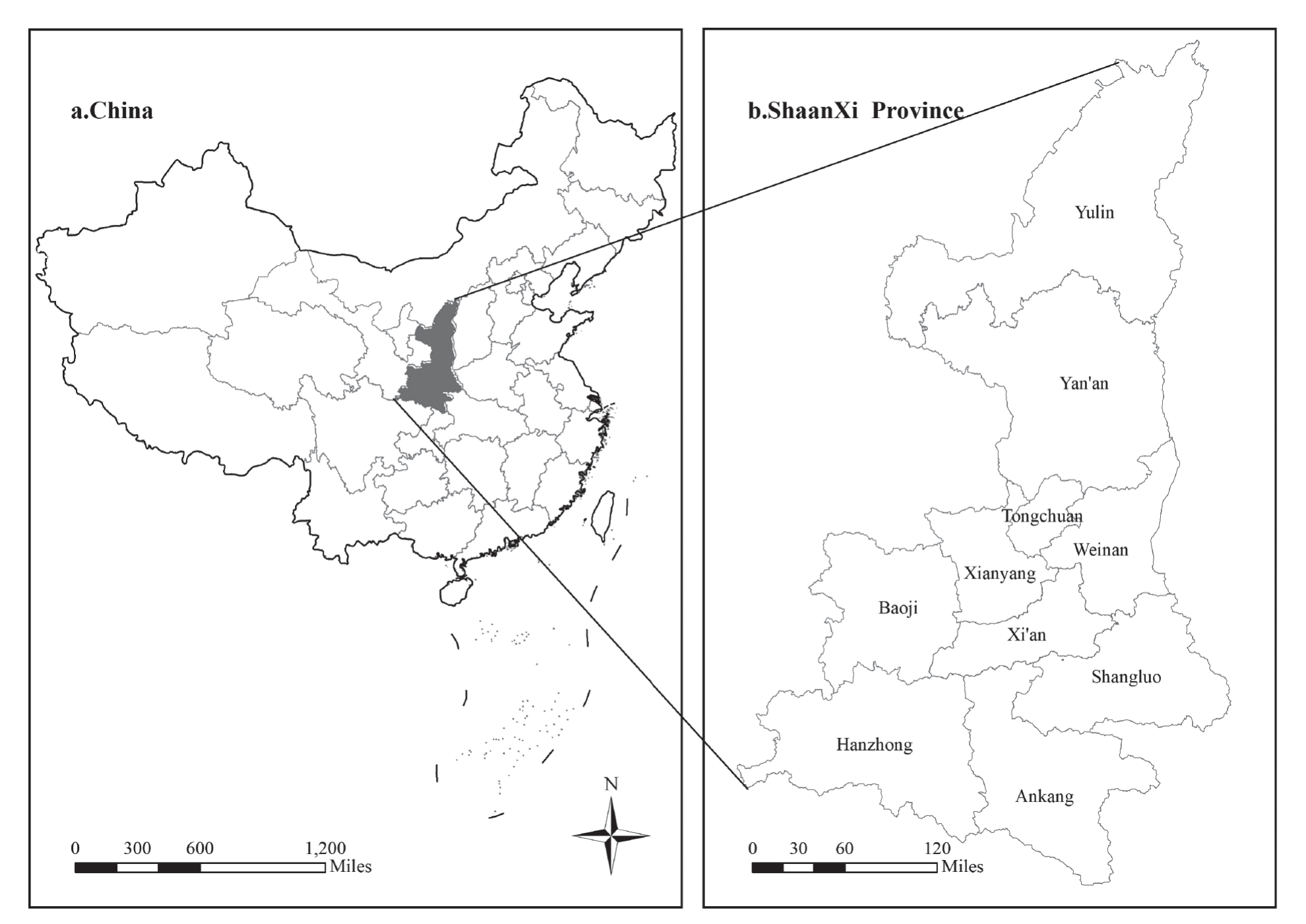
This study focuses on the transportation industry in Shaanxi Province, China. The transportation industry is not only a pillar industry in Shaanxi Province but also has a significant impact on the country’s social and economic development. At the same time, Shaanxi Province plays a crucial role as a major energy resource province in China with abundant oil, gas, and coal resources. Shaanxi Province is located in the Central Plains region and has always played an important role as a key transportation hub connecting northwest China to the world. The Silk Road is one of the most important trade routes in ancient and modern China. Shaanxi Province is located at the core of the Silk Road. This geographical location allows Shaanxi Province to play an important role in domestic and foreign trade exchanges, thereby contributing to the prosperity and development of the local economy. As the national economy rapidly develops and the Western Development Strategy is deeply implemented, Shaanxi Province will further strengthen cooperation and exchanges with other regions to enhance its comprehensive competitiveness. Due to the evident spatial variations in resources, population, economy, and industrial structure of various regions in Shaanxi Province, the specific measures for regional carbon emission reduction are also different. The results of carbon emission reduction in the region directly impact the achievement of China’s overall carbon reduction objec-tives. Hence, research on the carbon emissions of the transportation industry in this region can offer both theoretical and practical foundations for its emission reduction efforts. Fig. 1 is drawn through ArcMap software.
Material and Methods
Carbon Emission Calculation
There are no standardized calculation rules for the calculation of carbon emissions in the transportation industry. The transportation industry is vast, dispersed, and highly mobile, posing challenges for precise and accurate measurement of carbon emissions. Hence, scholars typically employ fuzzy estimation methods to calculate carbon emissions in the transportation industry. The carbon emission coefficient method proposed in the 2006 IPCC Guidelines for National Greenhouse Gas Inventories is used by many countries to calculate domestic carbon dioxide emissions. The carbon emission coefficient method is divided into two approaches: the “Top-down Approach” and the “Bottom-up Approach”. The “Top-down Approach” calculates carbon emissions based on the annual energy consumption in the transportation sector and the corresponding carbon emission factors. Because of the ease of data acquisition and the relatively accurate estimation results, numerous scholars have employed this method to assess carbon emissions in different regions. Liu et al. [43] calculate and analyze the current situation of urban traffic carbon emissions using various methods. Other scholars [44–46] use the “Top-down Approach” method to calculate carbon emissions from the transportation industry in each province and city in China. On the contrary, the “bottom-up” method calculates carbon emissions in the transportation industry based on refined data, including the type of vehicle, mileage, and energy consumption proportion. In comparison to the “Top-down Approach”, the “Bottom-up Approach” necessitates the collection of a broader range of basic data, increasing the difficulty of actual measurement. Ning et al. [47] estimated the carbon emissions from residential transportation in Zhengzhou City. Furthermore, some scholars integrate the two methods. Tian et al. [48] employed two combined methods to establish a transportation carbon emission measurement model with explicit statistical standards that can be benchmarked against international norms. They calculated the carbon emissions of China’s transportation industry and various modes of transportation in 2019.
This study employed the “Top-down Approach” to calculate the carbon emission data for the transportation industry in Shaanxi Province from 1995 to 2021. The carbon emissions calculation model of the transportation industry can be established using Equation (1).
In Equation (1), C is the total carbon emissions of the transportation industry; t is the type of energy; Ct is the carbon emissions of the t-th energy; λt is the carbon emission coefficient of the t-th energy source, which is the carbon dioxide produced by consuming unit energy; θt is the conversion coefficient of the t-th energy into standard coal, which is the amount of unit energy converted into standard coal; Et is the consumption of the t-th energy. The energy consumption data for the transportation industry in Shaanxi Province, China, can be obtained from the China Energy Statistical Yearbook. The data in this study were sourced from the web-site of the China Bureau of Statistics, the Shaanxi Statistical Yearbook, and the China Transportation Industry Statistical Yearbook from 1995 to 2021. Eight types of terminal energy consumption, including raw coal, crude oil, gasoline, kerosene, diesel, fuel oil, electricity, and natural gas, will serve as the basis for accounting for carbon emissions in the provincial transportation industry. As per the National Greenhouse Gas Inventory Guidelines issued by the IPCC in 2006, the carbon emission accounting coefficients are shown in Table 1.
Dual Feature Extraction
Spearman Coefficient
Due to the strong nonlinearity and complexity of carbon emission data, the Spearman coefficient suitable for nonlinear data is selected for the first feature selection. The calculation formula for the Spearman coefficient is shown in Equation (2):
In Equation (2), X and Y are two random features in the data set; RX and RY are the ranks of the X feature and Y feature, respectively; n is the number of features.
GBDT Model
This study employs the gradient boosting decision tree regression model for the second stage of feature selection. The gradient boosting decision tree is an ensemble learning algorithm that consists of multiple decision trees. The forward-distributed iteration method is mainly used to optimize the loss function by learning the base function and updating the weight coefficient in each iteration so that the algorithm can effectively handle the nonlinear relationship between features. In the gradient boosting decision tree model, feature contribution can be estimated by observing the contribution of features to the loss function in each iteration. Specifically, the gradient information (negative gradient) of each feature after each iteration can be used to estimate its contribution. Feature selection is performed by evaluating the contribution of features.
Define the model after the m – th round of iteration as Fm(x), and the loss function as L(y, Fm(x)). The negative gradient gim represents the negative gradient of the model for the actual label yj of sample i after the m-th iteration. The contribution of feature j to sample i after iteration m can be estimated by calculating the partial derivative of feature j.
The gradient j of feature for the sample i after the m-th iteration can be shown in Equation (3).
In Equation (3), xij is the j-th feature of sample i. The contribution degree gijm is further associated with the gradient gijm(m–1) of feature j in the previous iteration. The following results are obtained through the chain rule of Equation (4).
In Equation (4), gijm(m–1) is the gradient of feature j after (m-1) iterations. The second term of the formula on the right side represents the contribution of feature j to sample i due to changes in the model in the m-th iteration. This contribution can be accumulated through iterations. The contribution of feature in the GBDT model can be shown in Equation (5).
In Equation (5), M is the total number of iterations, and N is the number of training samples.
Pelican Optimization Algorithm
The POA was introduced in 2022 and is primarily com-posed of two phases: the exploration phase and the development phase. The algorithmic process is as follows:
First, initialize the pelican population.
In Equation (6), xij is the position of the i – th pelican in the j-th dimension; N is the population number of peli-cans; m is the dimension of the problem to be solved; rand is a random number in the range of [0,1]; the variables uj and lj are represent the upper and lower bounds for solving the J-dimensional problem.
After the initialization is completed, the pelican enters the exploration stage, generates the prey location randomly in the solution space, and moves toward the prey location. Its expression is shown in Equation (7).
In Equation (7), xP1ij is based on the j-th dimension position of the i-th pelican after the first stage update; I take on a random integer of 1 or 2; pj is the position of the prey in the j-th dimension; Fi is the objective function value of the i-th pelican; Fp is the objective function value of the prey.
In POA, the pelican accepts a new position if the objective function value at that position is better. The process is in Equation (8).
In Equation (8), Fp1i is the objective function value based on the new position of the i-th pelican updated in the first stage. After the exploration phase is completed, the pelican enters the development phase, converging toward better hunting positions. Its expression is in Equation (9).
In Equation (9), R is a constant with a value of 0.2; t is the current number of iterations, and T is the maximum number of iterations. In the development stage, when the optimal value is smaller, it is updated according to Equation (9).
In Equation (10), xp2i is the new position of the i-th pelican and Fp2i is the objective function value based on the second stage. As the number of iterations increases, the Pelican optimization algorithm also faces defects such as falling into local optimality. Therefore, the Pelican optimization algorithm is improved in the following aspects: therefore, the POA is improved in the following aspects, and the improved algorithm is called the IPOA.
Adaptive Weight
In the improvement of intelligent optimization algorithms, the introduction of weights can effectively improve the optimization accuracy of the algorithm. Therefore, linear weights are introduced in the exploration phase and development phase of the Pelican optimization algorithm, as shown in Equation (11).
Tent Chaos Mapping
Chaos has the characteristics of being random, non-repetitive, and ergodic. Chaos theory is introduced to improve the initialization phase of the algorithm to obtain an initial population uniformly distributed in the search space, which is beneficial to maintaining the diversity of the population, expanding the search range of the population, and improving the search performance of the algorithm. Tent mapping is used to initialize the population and expand the search range of the initial solution, as shown in Equation (12).
In Equation (12), X(m) is the chaos value.
The basic steps are:
Step 1: Randomly generate an n-dimensional matrix from 0 to 1 in the space, which is X(1);
Step 2: Iteratively generate the Tent chaos sequence of other individuals from the first individual X(1) according to the following formula:
Step 3: After obtaining all the solutions in the search space, map them to the original space again, as shown in Equation (13).
In Equation (13), Xn is the initial solution generated by the Tent chaos map, minn is the lower limit of the control variable, and maxn is the upper limit of the control variable.
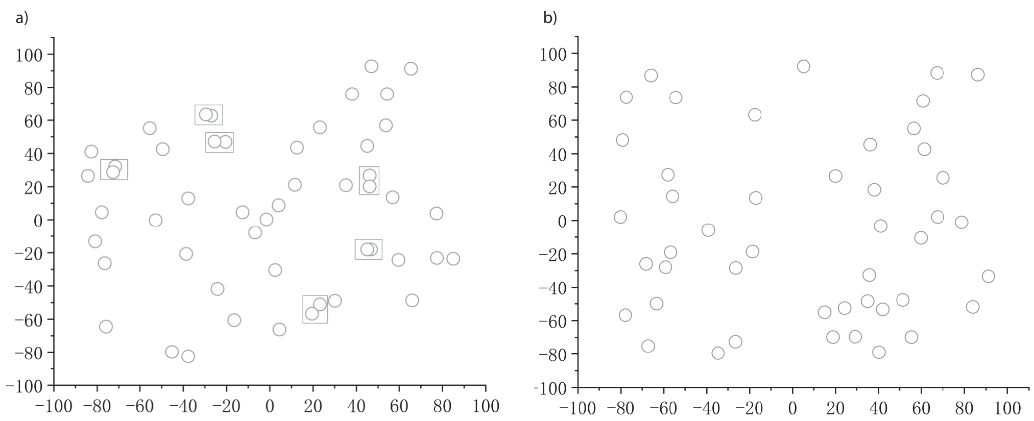
Fig. 2(a) shows the population distribution diagram generated by random initialization, and Fig. 2(b) shows the population distribution after using the Tent chaotic mapping model. It can be seen that the population is more dispersed in the mapped initialization distribution, and the number of individuals on the boundary and overlap-ping individuals is smaller. The wider distribution in the initialization stage can ensure the diversity of the population and reduce the attraction of local optimality.
Gaussian Mutation and Gaussian Perturbation
Gaussian variation refers to extracting a random number from the normal distribution with mean μ and σ2 variance and replacing the parameter variables in the POA algorithm to achieve the purpose of optimizing the algorithm. According to the distribution characteristics of the normal distribution curve, the main search range of a Gaussian mutation is a certain area near the original individual. Hence, the characteristics of the Gaussian mutation determine that it has strong local search capabilities, which is conducive to the algorithm finding global extreme points efficiently and accurately for optimization problems involv-ing multimodal functions. To this end, Tent chaos mapping and Gaussian mutation are combined to coordinate global search and local exploration capabilities, aiming to improve the convergence speed and evolution performance of POA. The Gaussian variation formula is shown in Equation (14).
In Equation (14), Tg is the value after Gaussian mutation of the original parameters; T is the original parameter variable; N(0,1) is a normal random distribution number with an expected value of 0 and a standard deviation of 1.
Gaussian perturbation. In order to improve POA’s ability to jump out of the local optimal solution, Gaussian micro-perturbation is performed on the individual optimal position after each iteration to help it better escape from the local optimal area. The Gaussian perturbation expression is shown in Equation (15).
In Equation (16), Gb is the optimal position of the pelican in each iteration; G is the fitness before Gaussian perturbation, Gaussian (μ, σ2) is a Gaussian function with mean μ and variance σ2; NGtb is the fitness value of the pelican individual after the disturbance; Gt is the optimal fitness of the pelican individual in the t – th iteration. After the population iteration is completed, new individuals are perturbed to speed up the convergence accuracy of the population. Hence, a Gaussian variation disturbance factor is used, which effectively prevents the population from falling into local optimality.
KELM Model
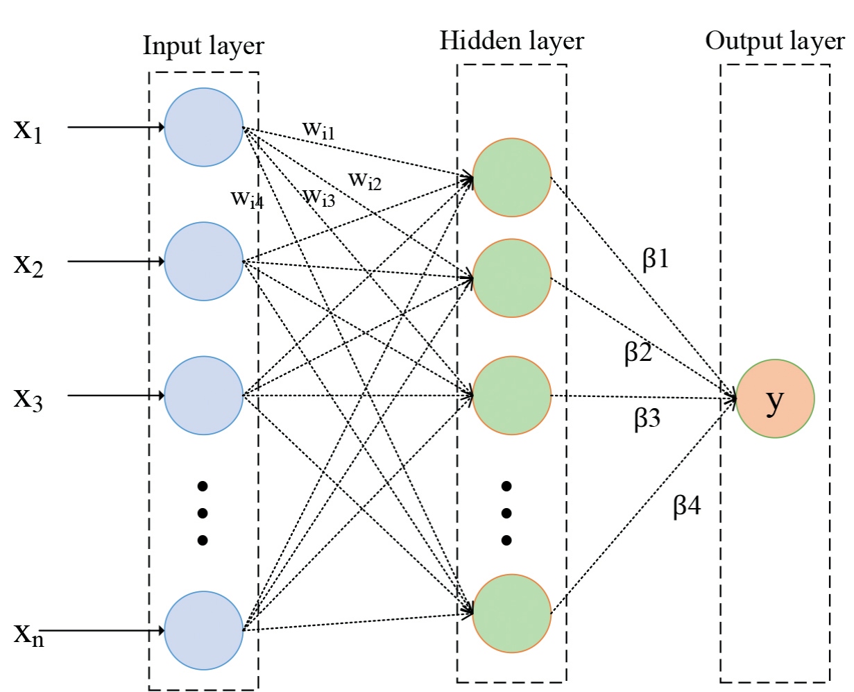
KELM is an improved algorithm proposed based on the Extreme Learning Machine (ELM) and combined with the kernel function. KELM can improve the prediction performance of the model while retaining the advantages of ELM. The ELM network structure is shown in Fig. 3.
ELM is a single hidden layer feedforward neural network, and its learning objective function can be expressed as a matrix.
In Equation (17), x is the input vector, h(x) and H are the hidden layer node outputs, β is the output weight, and L is the expected output.
Turning network training into a linear system solution problem, β is determined according to β = H * L, where H* is the generalized inverse matrix of H. In order to enhance the stability of the neural network, the regularization coefficient c and the identity matrix I are introduced, and then the least squares solution of the output weight is shown in Equation (18).
Introducing the kernel function into ELM, the kernel matrix is shown in Equation (19).
In Equation (19), xi, xj are test input vectors, then the above formula can be shown in Equation (20).
In Equation (20), (x1, x2, …, xn) is a given training sample, n is the number of samples, K is the kernel function, and c is the regularization coefficient. In summary, it can be seen that the kernel function parameter s and regularization coefficient c are important factors affecting the prediction performance of KELM.
DFE-IPOA-KELM Model Construction
Carbon Emissions Forecasting Process for the Transportation Industry
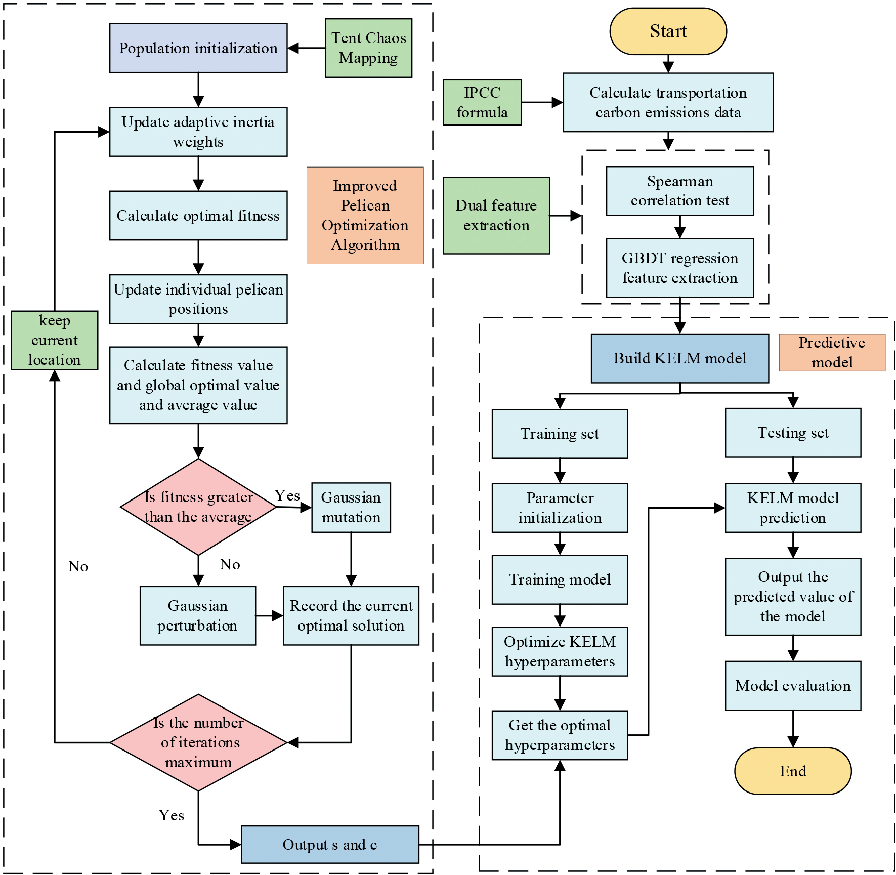
This study takes real carbon emission data from the transportation industry in Shaanxi Province, China, spanning from 1995 to 2021, as the experimental dataset. First, relevant data on carbon emissions in the transportation industry was collected according to the China Energy Statistical Yearbook, and its carbon emissions were calculated through the “Top-down approach” in the IPCC formula. Secondly, the Spearman coefficient and gradient boosting decision tree regression are used to select features that affect carbon emissions. The outcomes of feature selection are fed into the finalized KELM model for predicting carbon emissions. Finally, to enhance the prediction accuracy of the KELM model, this study will utilize the IPOA algorithm to optimize the KELM model, thereby creating a comprehensive prediction model. The model constructed is named DFE-IPOA-KELM. The specific algorithm flow is illustrated in Fig. 4.
The specific steps for prediction by the DEF-IPOA-KELM model are:
1. Input data.
Preprocessing the computed dataset involves outlier correction and normalization, as per Equation (17), trans-forming numerical values into the range of . This process eliminates dimensional differences to prevent significant errors caused by large differences in the magnitude of the input data. The initial 70% and the remaining 30% of the preprocessed dataset are segregated into training and test sets for the prediction model.
In Equation (21), is the minimum value in the influencing factor data sequence, is the maximum value in the sequence, is the initial input data, and is the data after normalization.
2. Initialize the improved Pelican optimization algorithm.
Add the Tent chaos map generate the initial pelican population, and calculate the population fitness. The pelican population location information is mapped to two hyper-parameter values of the KELM internal kernel function parameter and regularization coefficient c.
3. Update the individual locations of the pelican population.
Assign adaptive inertial weights to the initial population of IPOA, calculate the optimal fitness, and update the individual positions within the pelican population. Assess whether the fitness exceeds the average value. If it surpasses the fitness value, employ Gaussian variation to calculate the average fitness value at this time. In cases where fitness is below the average value, apply Gaussian perturbation to facilitate movement away from the optimal position. Keep a record of the current individual’s optimal solution and the global optimal solution until the maximum number of evolutions is attained.
4. Determine the number of iterations.
If the population reaches the maximum number of evolutions, the optimal parameters will be output and assigned to the KELM model. Otherwise, repeat steps (2–3).
5. The DFE-IPOA-KELM model
Establish a complete DFE-IPOA-KELM prediction model and conduct experimental comparative analysis using proportionally divided data sets.
Results
Data Description
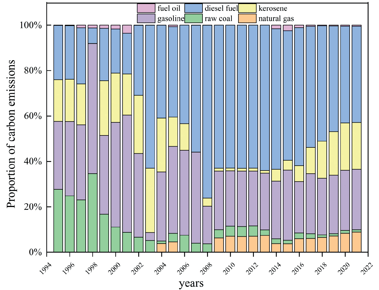
Regarding energy consumption in the transportation industry in Shaanxi Province, petroleum products constitute the predominant share. Consequently, carbon dioxide emissions from this type of energy significantly influence the overall carbon emission structure of the transportation industry. Fig. 5. illustrates that the proportion of carbon dioxide generated by oil energy consumption has risen from 72.3% in 1995 to 90.1% in 2021, whereas carbon dioxide emissions from coal have decreased from 27.7% in 1995 to approximately 1% in 2021. As natural gas was not extensively utilized before 2003, the carbon emissions from natural gas during this period were not incorporated into the total carbon emissions in the transportation industry for that year. Despite the gradual promotion of clean energy by the Chinese government and enterprises since 2003, leading to a rise in the proportion of carbon emissions to 8.9% by 2021, the primary source of carbon emissions in the transportation industry remains the consumption of fossil energy. A potential reason for this issue is the continued economic development of Shaanxi Province following western China’s development. Simultaneously, enhancements to the transportation system and the diversi-fication of transportation modes have facilitated increased regional exchanges, leading to a rapid upsurge in energy consumption in the transportation industry.
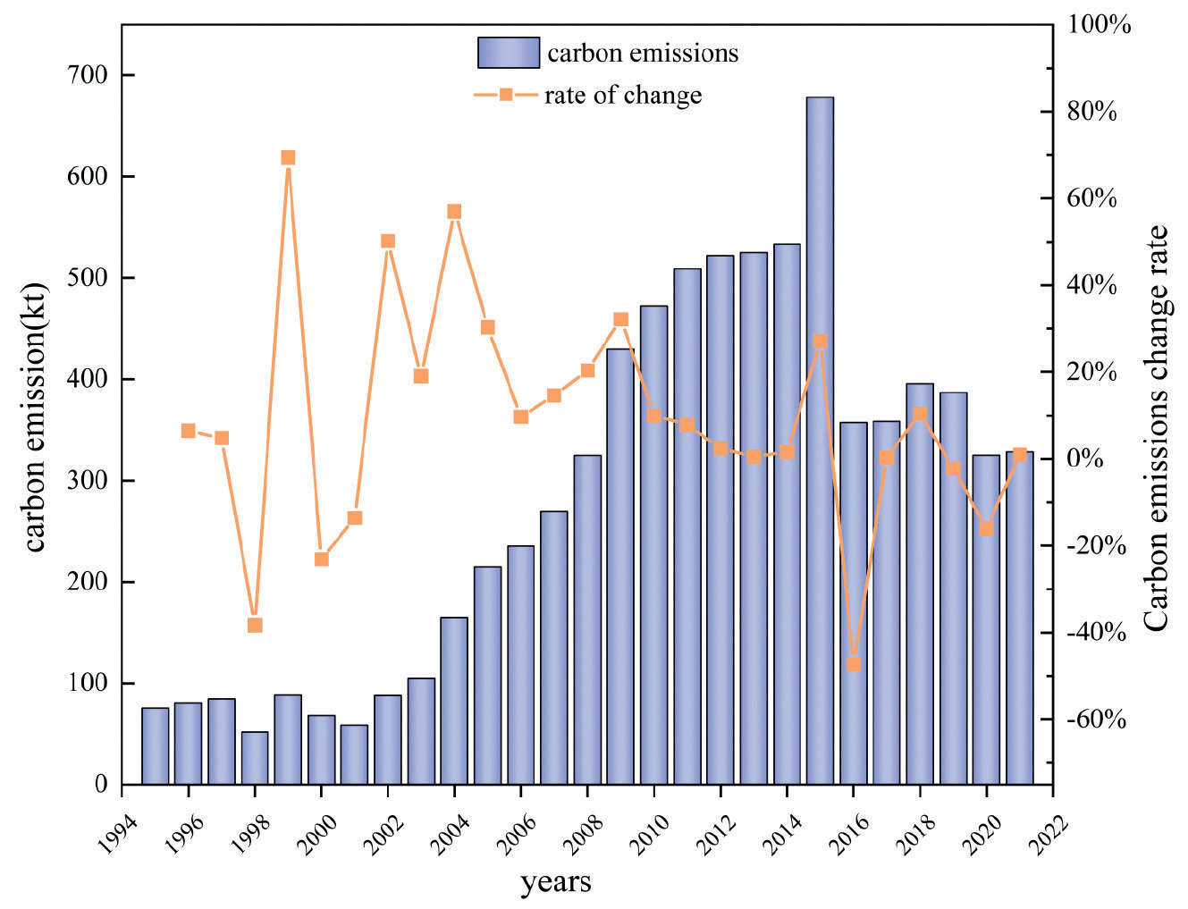
The evolution of total carbon emissions from the transportation industry in Shaanxi Province can be delineated into three stages, as shown in Fig. 6. Before 2000, the region’s carbon emissions fluctuated around one million tons. This fluctuation can be attributed to the transportation industry’s relatively modest development during this period, resulting in lower energy consumption demands. From 2001 to 2015, driven by the accelerated urbanization process and the in-depth advancement of the Western Development Project, the transportation industry in Shaanxi Province entered a stage of rapid expansion. In this period, the consumption of fossil energy led to an explosive growth in carbon emissions from the transportation industry. Due to the effective implementation of the carbon emission reduction strategy and the gradual adoption of low-carbon development initiatives by the Shaanxi provincial government, carbon emissions in the transportation industry subsequently plummeted, dropping below four million tons in 2016. However, in recent years, the overall carbon emissions from the transportation sector in Shaanxi Province have remained elevated compared to the initial stage.
Dual Feature Extraction
Based on the energy consumption characteristics of the transportation industry among provinces, this study selected the urbanization rate (U), GDP, transportation gross product value (TGDP), energy intensity (EI), energy consumption (EC), energy structure (ES), population (P), vehicle ownership (VO), passenger volume (PV), freight volume (FV), passenger turnover (PT), and cargo turnover (CT). These 12 variables serve as the main factors affecting carbon emissions in the transportation industry.
The thoughtful selection of input parameters is crucial for establishing a carbon emission prediction model. To enhance prediction accuracy, it is essential to extract the features of influencing factors before inputting prediction data. The initial step involves utilizing the Spearman correlation coefficient to calculate the relationship between relevant explanatory variables and transportation carbon emissions (C), as well as the correlation between each explanatory variable. Retaining factors are strongly correlated with carbon emissions, and highly correlated variables are eliminated. Subsequently, the gradient boosting decision tree regression method is applied to calculate the contribution of each feature in the original data to affecting carbon emissions.
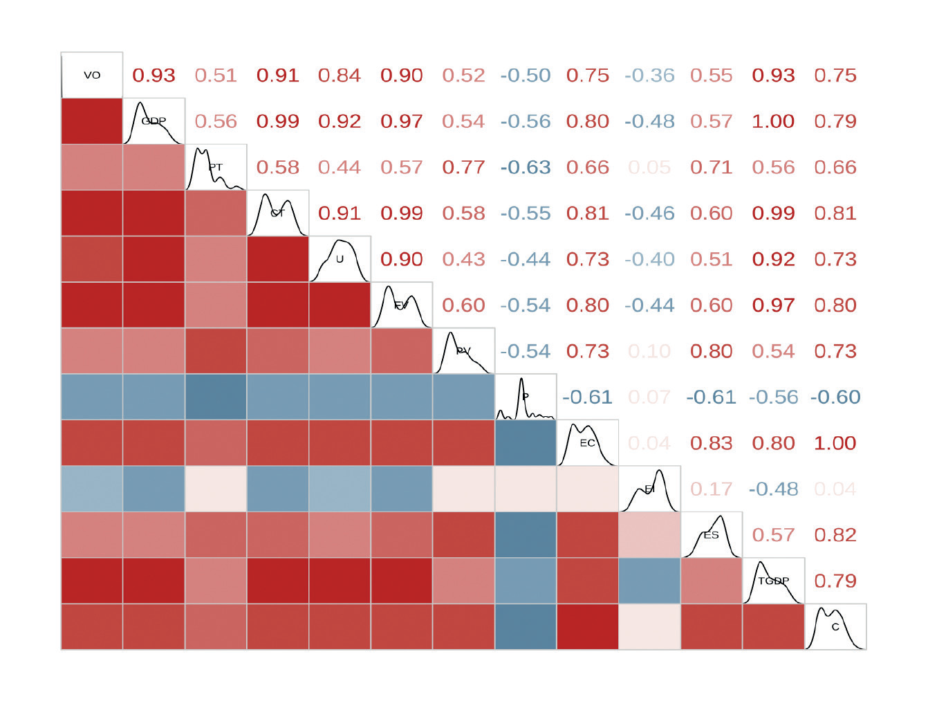
The analysis results of the Spearman correlation coefficient are shown in Fig. 7, which reveal that eight factors: TGDP, ES, EC, FV, CT, U, GDP, and VO have correlation coefficients exceeding 0.7. This indicates that these factors exhibit a strong positive correlation with carbon emissions in the transportation industry, implying a significant impact on carbon emissions.
To mitigate the potential bias from a single method on feature selection, the gradient boosting decision tree was used to further calculate the contribution of each influencing factor to carbon emissions. As depicted in Fig. 8, the greater the contribution of each factor, the more significant its impact on carbon emissions in the transportation industry. According to the gradient boosting decision tree regression results, the top six con-tributors to carbon emissions are as follows: energy structure contributes 29.4% to carbon emissions, energy consumption accounts for 18.8%, freight turnover accounts for 15.9%, and transportation industry The contribution of GDP and urbanization rate were 12.5% and 9%, respectively, and the contribution of the number of motor vehicles reached 10.2%.
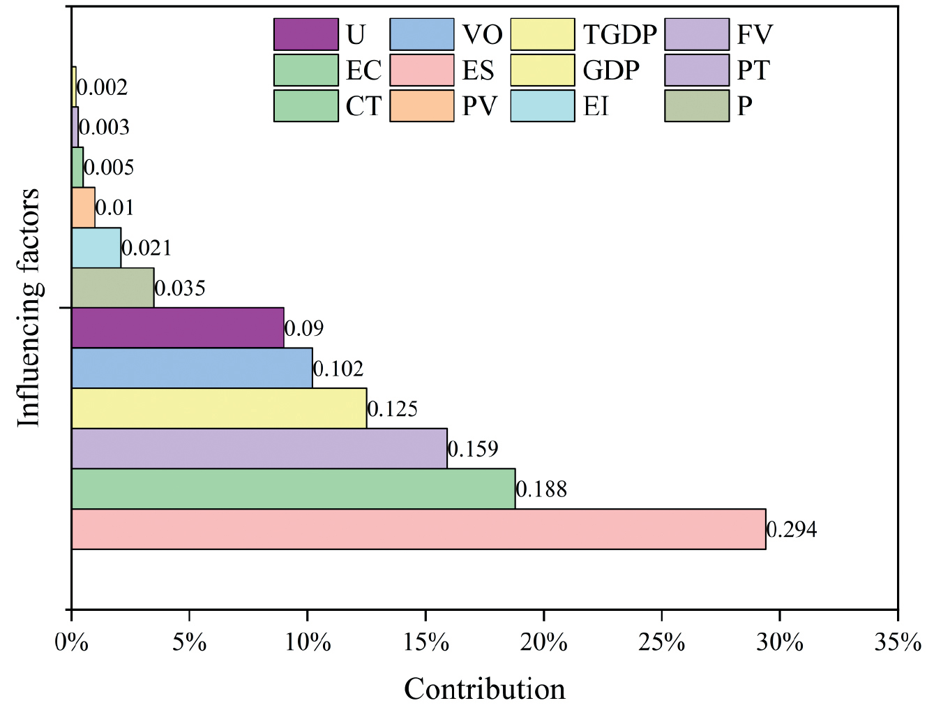
Through cross-comparing the Spearman coefficient and GBDT contribution, the TGDP, EC, ES, VO CT, and U were identified as predictors of carbon emissions from the transportation industry, as shown in Table 2.
Model Evaluation Index
To assess the prediction effectiveness of the proposed combination model, this study employed the root mean square error (Root Mean Square Error, RMSE), the mean absolute error value (Mean Absolute Error, MAE), and the mean absolute percentage error (Mean Absolute Percentage Error, MAPE) as the evaluation index to quantify the difference in error between predictions and ground truth variables. The specific calculation formula is as follows: In general, a higher value and a lower RMSE/ MAE/MAPE value indicate better estimation performance of the model.
Where η̂k is the predicted value; ηk is the real value.
Configuration of Model Parameters
In this study, the MATLAB R2022A software platform will be used to verify the prediction effect of the proposed DFE-IPOA-KELM model. The training set and test set data are divided according to the 7:3 ratio. After repeated training of the model, the DFE-IPOA-KELM model works best when the pelican population is set to 30, and the maximum number of iterations is 50. Therefore, in this study, the population size of IPOA and POA was standardized to 30, and the maximum number of iterations was uniformly set to 50. Five models, namely KELM, SSA-KELM, PSO-KELM, POA-KELM, and IPOA-KELM, were employed for comparative analysis. To ensure the comparability of the experiment, the configuration of these five models is standardized: the number of input layer neurons is set to 6, the number of hidden layer neurons is set to 9, the number of output layer neurons is 1, and the number of training times and accuracy requirements remains consistent. Specifically, the number of training times is set to 500, and the accuracy target is 0.001. On the training set, the trend changes in the fitness of four algorithms, SSA, PSO, POA, and IPOA, are shown in Fig. 9. The search range of the kernel function parameter (s) is set to [10-2, 10], and the search range of the regularization coefficient (c) is set to [10-2, 102]. Through multiple experiments, the parameter results optimized by different algorithms are averaged and input into the KELM model. The optimal kernel function parameters and regularization coefficient for different model structures are shown in Table 3.
Comparative Analysis of Predictive Outcomes
Based on the model parameters set in the previous steps, input the preprocessed data and iteratively train the model. The comparison curve between the predicted value and the actual value of each model is shown in Fig. 10. The relative error curves calculated for various comparison models are shown in Fig. 11.
The results of the DFE-IPOA-KELM model on the test set sample data show that this model is better than other control models in predicting carbon emissions in the transportation industry. The suboptimal fitting performance of the standalone KELM prediction model indicates its effect is not ideal. Likewise, the fitting performance of the KELM model, even after optimization through the algorithm, remains subpar. Essentially, the predicted values from both model structures display a significant deviation from the actual values, indicating a low level of accuracy. The prediction results of various model structures are shown in Table 4, which represents the relative error value. Simultaneously, by combining Fig. 11 and Table 5, it is evident that the DFE-IPOA-KELM model exhibits the smallest relative error value, with an average relative error of only 2.51%. The average relative errors for KELM, POA-KELM, and IPOA-KELM are 9.82%, 5.91%, and 4.12%, respectively. The average relative errors of the DFE-IPOA-KELM model are lower than those of the other three control models, once again affirming that the model has higher prediction accuracy.
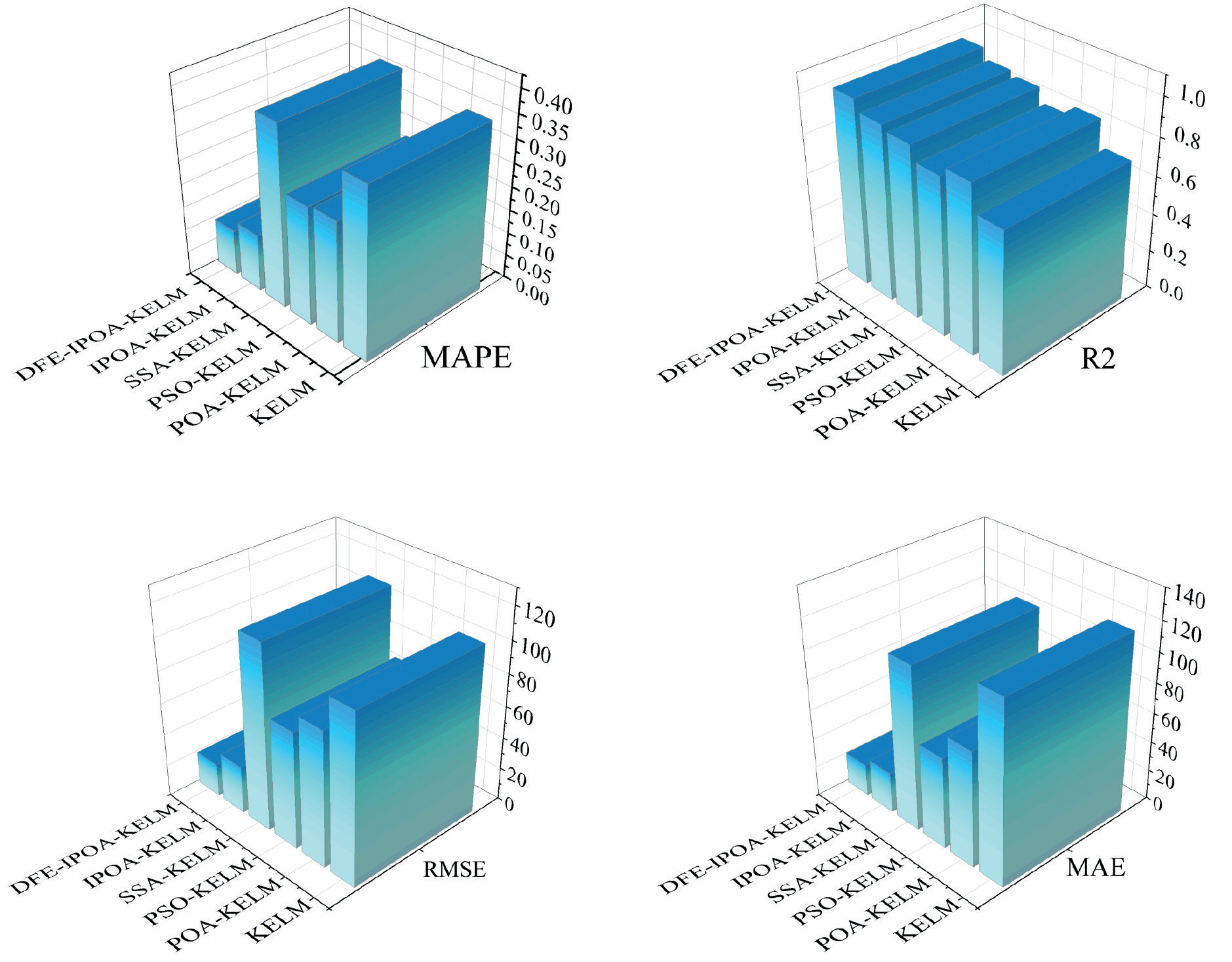
The analysis of error indicators for predicting transportation industry carbon emissions for different models is visually displayed in Table 5 and Fig. 12. The RMSE of DFE-IPOA-KELM is 94.06, 51.90, 9.15, 63.09, and 84.16 lower than SSA-KELM, PSO-KELM, IPOA-KELM, POA-KELM, and KELM, respectively. The for the model proposed in the research is 97.75%, surpassing that of the other three control models. Simultaneously, MAPE and MAE outperform the other five models. Comparing KELM, SSA-KELM, PSO-KELM, POA-KELM, IPOA-KELM, and DFE-IPOA-KELM, it is evident that the prediction model utilizing the gradient boosting decision tree for feature selection combined with the IPOA significantly influences the transportation industry. The carbon emissions prediction accuracy is superior, indicating minimal deviation of the model’s predicted values from the true values. Therefore, DFE-IPOA-KELM outperforms traditional KELM and the singly optimized KELM prediction model, demonstrating greater stability and robustness.
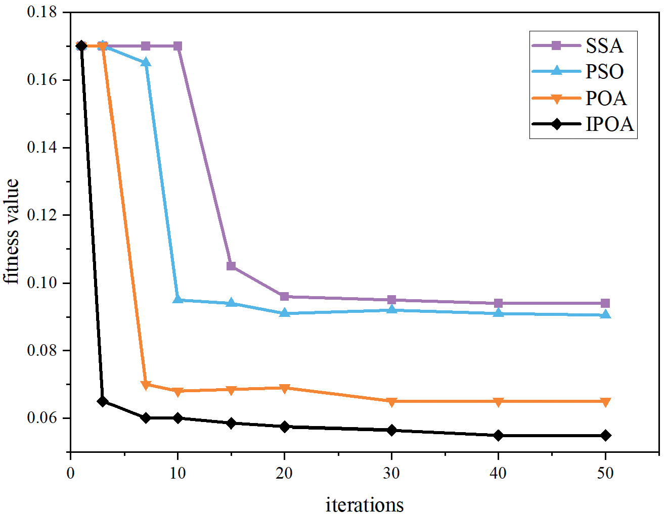
Table 3.
Optimal Parameters for Various Models.
| Model | parameter | optimal value |
|---|---|---|
| KELM | s | 0.06 |
| c | 89.21 | |
| POA-KELM | s | 0.08 |
| c | 100.00 | |
| PSO-KELM | s | 0.21 |
| c | 81.36 | |
| SSA-KELM | s | 0.46 |
| c | 71.59 | |
| IPOA-KELM | s | 1.18 |
| c | 65.32 |
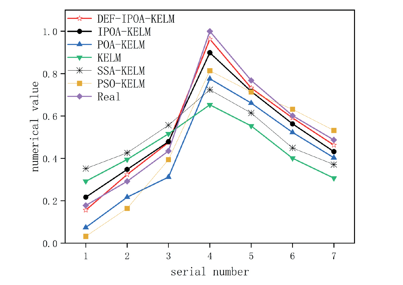
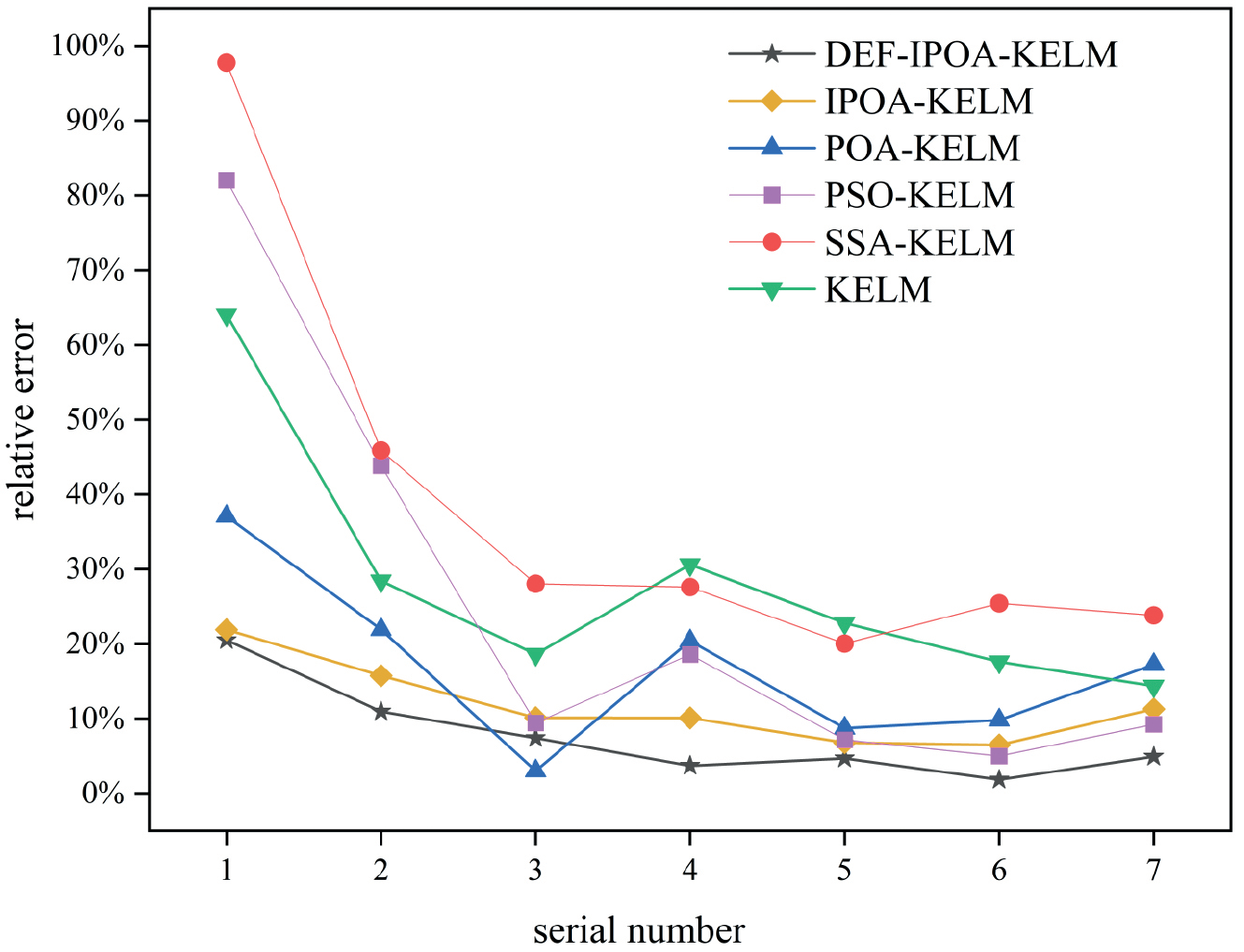
Table 4.
Test Results of Model Data.
The above experimental results demonstrate that the DFE-IPOA-KELM model exhibits superior prediction accuracy compared to the KELM, POA-KELM, PSO-KELM, SSA-KELM, and IPOA-KELM models. On one hand, the improved prediction performance of the proposed model can be attributed to the introduction of kernel functions and optimization processes into the extreme learning machine, effectively addressing the issues of reduced generalization and stability caused by the random assignment of hidden layer neurons. On the other hand, gradient boosting decision tree regression is employed to conduct feature screening on the dataset, minimizing the ef-fects of multicollinearity between indicators. Hence, DFE-IPOA-KELM can serve as an effective model for carbon emission prediction research in the transportation industry.
Scenario Simulation
Scenario Setting
In this study, we will consult pertinent policy reports and data releases from the Shaanxi Provincial Government to establish distinct rates of change for factors influencing carbon emissions in the transportation industry. As shown in Tables (6-7), different changing rates of influencing factors correspond to different carbon emission scenarios. This study will conduct scenario forecasts of carbon emissions from the transportation industry from 2022 to 2040. To make the prediction process more consistent with the actual situation and the prediction results more scientific and reasonable, this study will set up four stages to predict the future carbon emissions of the transportation industry in Shaanxi Province.
Table 5.
Comparison of model performance evaluation indexes.
The six influencing factors identified above in this study are used as research objects for future carbon emissions from the transportation industry in Shaanxi Province. The change rate of factors affecting carbon emissions is determined by national policies, national development plans, and the research results of relevant scholars.
Gross Domestic Product of the Transportation Industry. From 1995 to 2021, the GDP of Shaanxi Province’s transportation industry increased at an average annual rate of 3.34%; it has risen from 7.792 billion yuan in 1995 to 124.717 billion yuan in 2021. During the “Thirteenth Five-Year Plan” period, Shaanxi Province completed a total of 460 billion yuan in transportation investment, an increase of 15% compared with the “Twelfth Five-Year Plan” period. The “14th Five-Year Plan” proposes that the province’s comprehensive transportation corridors will be basically completed by 2025. The network layout will be more optimized, and the coverage rate of high-efficiency transportation infrastructure will reach 100%. The change rate of the GDP of the transportation industry under different scenarios in the future is shown in Table 8.
Table 6.
Carbon emission scenario description of the transportation industry.
Table 7.
Change rate of carbon emission factors in the transportation industry.
| scenario | rate of change | |||||
|---|---|---|---|---|---|---|
| ES | EC | CT | TGDP | VO | U | |
| Baseline scenario | Low | Low | High | High | Low | High |
| Energy saving scenario | Middle | Middle | Middle | Middle | Middle | Middle |
| Low carbon scenario | High | High | High | Middle | High | Low |
Table 8.
Change rate of GDP in the transportation industry.
| rate of change | GDP of the transportation industry | |||
|---|---|---|---|---|
| 2022–2025 | 2026–2030 | 2031–2035 | 2036–2040 | |
| High | 5.96% | 4.26% | 3.42% | 2.96% |
| Middle | 4.65% | 3.55% | 2.15% | 1.92% |
| Low | 3.37% | 2.48% | 1.14% | 0.91% |
Cargo turnover. During the “Thirteenth Five-Year Plan” period, the average annual growth rate of freight turnover was 7.21%. From the perspective of category characteristics, bulk material transportation has grown steadily, and demand for small-batch and multi-frequency logistics has grown rapidly. From the perspective of mode characteristics, the transportation volume of railways and aviation will steadily increase, especially the proportion of bulk cargo and medium and long-distance cargo railway transportation will further increase, and the transportation structure will continue to be optimized. The rationalization of cargo transportation is gradually improving, and it is expected that freight turnover will show a slight downward trend after the “14th Five-Year Plan”. The future change rate of urbanization under different scenarios is shown in Table 9.
Urbanization rate. According to the goals of the “14th Five-Year Plan”, the urbanization rate of the province’s per-manent population will reach about 65% by 2025. During the “14th Five-Year Plan” period, China’s urbanization rate is expected to increase by an average annual rate of 1.03%. Compared with the “13th Five-Year Plan” period, it de-clined during the Five-Year Plan period. The growth rate of China’s urbanization development will begin to slow down during the “14th Five-Year Plan” period and will show a relatively stable trend after 2035. The change rate of urbanization under different scenarios in the future is set as shown in Table 10.
Energy consumption. According to the long-term goals of the “14th Five-Year Plan”, the province’s raw coal, crude oil, and natural gas production will reach 740 million tons, 27 million tons, and 36 billion cubic meters, respectively, by 2025. “Air Quality Standards Compliance Plan (2023-2030)” Shaanxi Province’s transportation industry energy consumption increased rapidly during the period 2021-2030, and the growth rate slowed down after 2030 with an average annual growth rate of 1.1%. The changing rates of energy consumption under different scenarios in the future are shown in Table 11.
Table 9.
Change rate of cargo turnover.
| rate of change | cargo turnover | |||
|---|---|---|---|---|
| 2022–2025 | 2026–2030 | 2031–2035 | 2036–2040 | |
| High | 3.8% | 3.1% | 2.4% | 1.5% |
| Middle | 3.5% | 2.8% | 2.1% | 1.3% |
| Low | 3.2% | 2.6% | 1.9% | 0.9% |
Table 10.
Change rate of urbanization.
| rate of change | urbanization rate | |||
|---|---|---|---|---|
| 2022–2025 | 2026–2030 | 2031–2035 | 2036–2040 | |
| High | 1.29% | 1.12% | 0.96% | 0.65% |
| Middle | 1.16% | 0.95% | 0.81% | 0.50% |
| Low | 0.98% | 0.78% | 0.65% | 0.35% |
Table 11.
Change rate of energy consumption.
| rate of change | energy consumption | |||
|---|---|---|---|---|
| 2022–2025 | 2026–2030 | 2031–2035 | 2036–2040 | |
| High | -4.24% | -2.14% | -1.98% | -1.65% |
| Middle | -4.11% | -3.79% | -1.71% | -1.42% |
| Low | -5.26% | -2.29% | -2.12% | -1.09% |
Table 12.
Change rate of energy structure.
| rate of change | energy structure | |||
|---|---|---|---|---|
| 2022–2025 | 2026–2030 | 2031–2035 | 2036–2040 | |
| High | -3.24% | 2.26% | -1.82% | -0.92% |
| Middle | -3.74% | -3.08% | -2.48% | -0.16% |
| Low | -4.18% | -2.61% | -2.19% | -1.29% |
Energy structure. The average annual growth rate of the energy structure from 2000 to 2019 was 7.6%. The Outline for Building a Powerful Transportation Nation proposes to “optimize the transportation energy structure, promote the application of new energy and clean energy, and promote all urban public and urban logistics distribution vehicles to be electrified, new energy and clean.” The rate of change of the energy structure under different scenarios in the future is shown in Table 12.
Motor vehicle ownership. According to the average annual change in motor vehicle ownership in Shaanxi Province from 1995 to 2021 of 2.3%, the number of civil-ian vehicles had reached 8 million by the end of 2020, and the average annual maximum change did not exceed 2.5%. The change rates of motor vehicle ownership under different scenarios in the future are shown in Table 13.
Multi-Scenario Forecast Results
The trained DFE-IPOA-KELM model is used to predict carbon emissions in the transportation industry from 2022 to 2040. This work uses this model to study the carbon emissions, peak value, and peak time of the transportation industry during this period. Based on the above scenario settings, the trained DFE-IPOA-KELM model is used to predict transportation carbon emissions in Shaanxi Province year by scenario. The carbon emissions from the transportation industry in Shaanxi Province from 2022 to 2040 under the three scenarios of baseline, energy saving, and low carbon are shown in Fig. 13.
Table 13.
Change rate of motor vehicle ownership.
| rate of change | motor vehicle ownership | |||
|---|---|---|---|---|
| 2022–2025 | 2026–2030 | 2031–2035 | 2036–2040 | |
| High | 2.21% | 2.41% | 2.01% | 1.70% |
| Middle | 2.05% | 2.25% | 1.85% | 1.50% |
| Low | 1.95% | 1.95% | 1.55% | 1.25% |
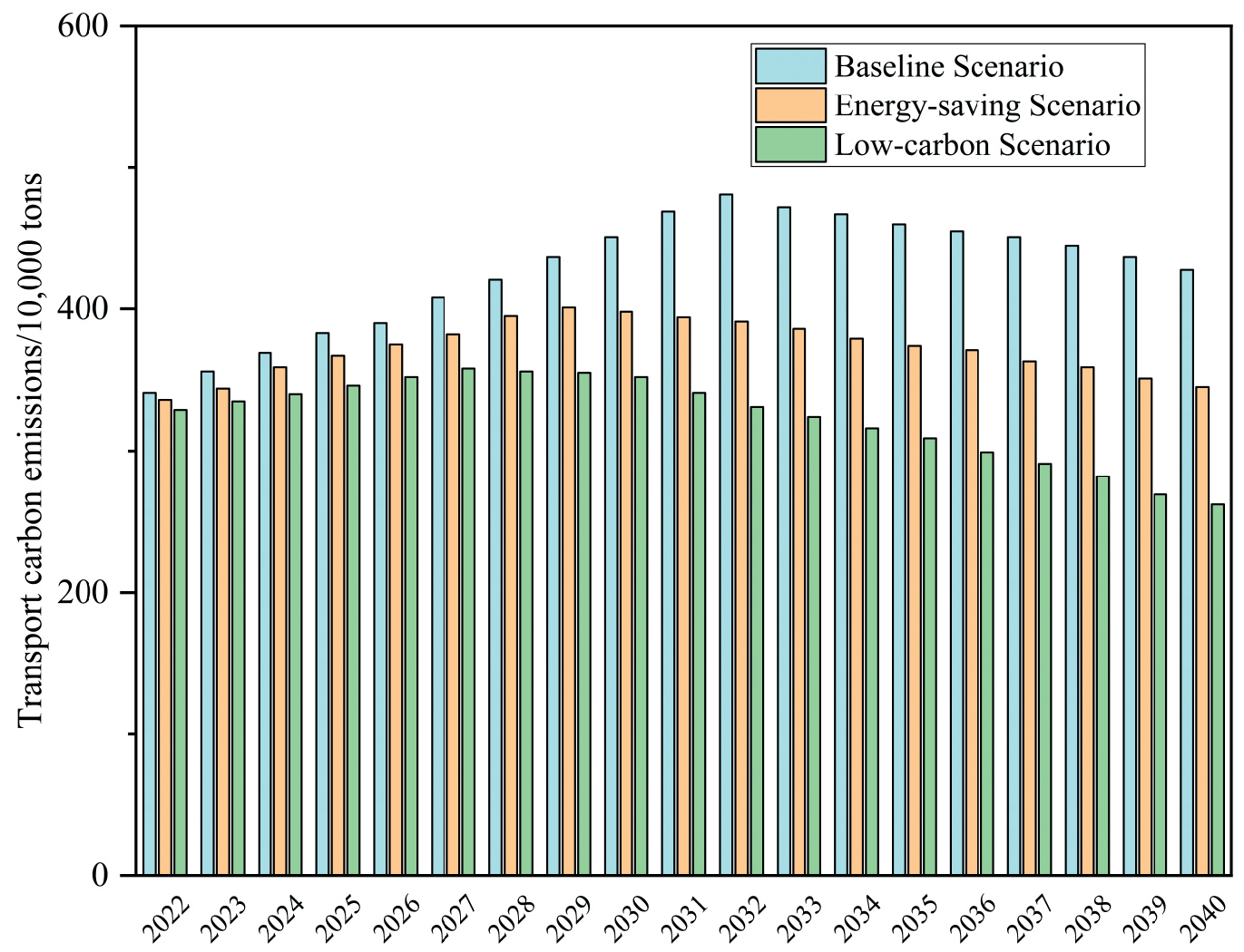
The prediction results show that after reaching their peak of carbon emissions, carbon emissions from the transportation industry in Shaanxi Province will gradually show a slow downward trend in the future. Under different scenarios, the peak value of carbon emissions in the transportation industry is different, and the time to reach the peak is also different. Under the baseline scenario, carbon emissions from the transportation industry will only reach a peak in 2032 and peak at 4.81 million tons. Under current social and economic development, the peak carbon emissions of the transportation industry in Shaanxi Province are more realistically reflected in this scenario. Under the energy-saving scenario, the carbon emissions of the transportation industry in Shaanxi Province will peak at 4.01 million tons of carbon emissions in 2029. This scenario focuses on the optimization of the energy structure and the improvement of energy efficiency and promotes the development of the transportation industry through the formulation of relevant policies. Under the low-carbon scenario, carbon emissions from the transportation industry in Shaanxi Province will peak at 3.58 million tons in 2027. Under this scenario, the transportation industry will gradually carry out energy-saving and green development through energy structure optimization and industrial structure adjustment. Comparative analysis of the three scenarios shows that the peak carbon emissions of the low-carbon scenario are 34.36% and 19.95% lower than the baseline scenario and the energy-saving scenario, respectively, and the peak time is also earlier. After peaking in 2027, carbon emissions under the low-carbon scenario show a more obvious downward trend.
Discussion
Our study shows that Shaanxi Province’s transportation industry is likely to achieve its carbon peak target in 2027 under a low-carbon scenario. However, under the baseline scenario, the transportation industry in Shaanxi Province will reach its carbon peak in 2032. The use of fossil energy has led to a sharp increase in carbon dioxide emissions, which has put tremendous pressure on environmental protection. According to the prediction results, it is not difficult to find that in Shaanxi Province’s transportation industry, to achieve the goal of carbon peaking before 2030, corresponding low-carbon measures must be taken to promote carbon emission reduction work.
The transportation industry in China’s regional sector constitutes a complex, large, and highly mobile system, and the carbon emissions it generates are also a complex system problem. Therefore, it is difficult to consider care-fully in the study of this article, and some factors need to be ignored. This study measures carbon emissions from the transportation industry; it only calculates direct carbon emissions based on the industry’s fossil energy consumption. However, in recent years, the widespread use of new energy vehicles in China has caused the transportation industry to indirectly produce a portion of carbon dioxide emissions. For example, the manufacturing and use of new energy vehicles will generate a large amount of electricity consumption, which will also indirectly increase carbon dioxide emissions from the transportation industry. In addition, this study ignores carbon emissions from fixed places such as stations, terminals, and airports. The lack of this important data may lead to certain deviations in the measurement results of the industry’s carbon emissions. In the prediction model training stage, due to missing data in some years, the amount of data used for model training in this study is limited, which may affect the prediction accuracy.
This study conducts modeling and policy simulation of the transportation industry’s carbon emission system to better describe the development process of the transportation industry’s carbon emissions and help the Shaanxi provincial government formulate a scientific and effective carbon emission control plan. However, the issue of transportation carbon emissions is a complex one. How to better simulate the transportation carbon emission system in conjunction with carbon emission reduction policy requirements still requires further in-depth research. At the same time, follow-up research will refine the spatial scale of the research object. We hope to use more detailed indicators to study the specific situation of transportation carbon emissions to make the research results more tar-geted. In the future, this research will focus on strengthen-ing the collection and statistics of mileage data for electric vehicles, and it is very meaningful to calculate their electric energy consumption. How to quantify the impact of new energy vehicles on carbon dioxide emissions from China’s transportation industry will be a research direction and hot spot in the future.
Conclusions
This study proposes a model based on dual feature extraction and an improved Pelican algorithm to optimize the kernel extreme learning machine. This model has high prediction accuracy and can more accurately describe the future carbon emission trend of the transportation industry in Shaanxi Province. This work first conducts a double screening of factors affecting carbon emissions in the transportation industry and adds macro-indicators that have an impact on carbon emissions as input variables of the prediction model. Secondly, by comparing the total carbon emission prediction results and error indicators of different models from 1995 to 2021, the advantages of the DFE-IPOA-KELM prediction model are proven. This article draws the following conclusions:
1. The DFE-IPOA-KELM prediction model constructed in this article has the minimum error-index value. Compared with the KELM, SSA-KELM, PSO-KELM, POA-KELM, and IPOA-KELM models, the RMSE, MAE, and MAPE of this model dropped to 20.63, 21.57, and 9.81%, respectively, and the R2 increased to 97.75%. The prediction accuracy of this model is better and is suitable for carbon emission prediction in the transportation industry.
2. The trained DFE-IPOA-KELM model is used to predict the carbon emissions of the transportation industry in three scenarios: baseline, energy saving, and low carbon. The predicted peak carbon emission results under the three scenarios are 4.81 million tons, 4.01 million tons, and 3.58 million tons, respectively, and the peak times are 2032, 2029, and 2027, respectively. According to the prediction results of the scenario simulation, the total carbon emissions from the transportation industry in Shaanxi Province will continue to increase until 2032. Therefore, in order to realize the carbon emission reduction commitment and reach the peak of carbon emissions as soon as possible, corresponding measures need to be taken to reduce total carbon emissions and actively respond to global warming.
Based on the factors influencing carbon emissions in the transportation industry proposed in this article and the prediction results of the above model, to enable the transportation industry in Shaanxi Province to achieve the carbon peak goal as soon as possible, the following policies and suggestions are put forward.
1. Focus on promoting the adjustment of the energy structure and recommend the use of clean energy. The huge consumption of fossil energy is the main factor affecting transportation carbon emissions. To alleviate the exces-sive use of primary energy, low-carbon technologies, and clean energy should be used as much as possible to promote the development of green transportation while ensuring the basic needs of transportation. On the other hand, we will improve relevant incentive policy systems and strengthen the trend toward low-carbon and high-quality development of related transportation equip-ment in the transportation field.
2. Promote urbanization rationally and reduce the pressure on land and resources caused by urban expansion. Based on the steady economic improvement of Shaanxi Province, urban residents’ awareness of low-carbon environmental protection will be gradually improved, and the concept of green and low-carbon travel will be cultivated. Finally, technological progress and in-novation related to energy conservation and emission reduction should be vigorously encouraged.
3. Carbon dioxide capture and storage (CCUS) technology is one of the key technologies to achieve low-carbon transformation of fossil energy and cope with climate change. China’s CCUS/CCS technology started late, so relevant policies should be actively introduced to support the development of carbon capture and other technologies to achieve the rapid development of CCUS technology in China.
Through policy adjustments, Shaanxi Province should focus on the main factors affecting carbon emissions in the transportation industry, so as to achieve the goal of peaking carbon emissions in the transportation industry as soon as possible.