

Introduction
As the ties between China and Russia deepen, their collaboration in trade, particularly in agriculture, has witnessed significant growth [1]. Both nations, being major players in the global agricultural market, have strengthened their trade relations due to factors like their entry into the World Trade Organization, the initiation of the Belt and Road Initiative, and economic sanctions imposed by Western countries on Russia [2]. This has led to a substantial increase in bilateral agricultural trade, reaching a total value of 5.5 billion USD in 2020, marking a sevenfold rise since 20011. China has emerged as the largest importer of Russian agricultural products, while Russia holds the third position among importers of Chinese agricultural goods [3].
The traded agricultural products are diverse, with China exporting processed items like vegetables, fruits, fish, crustaceans, and mollusks to Russia, while Russia exports 1 https://www.statista.com/statistics/1003171/russia-value- -of-trade-in-goods-with-china/ frozen fish, plant wood, soybeans, and edible oils to China. This comprehensive range of traded products showcases strong complementarity, positioning both nations as crucial partners in agricultural trade cooperation.
Amidst global economic growth, heightened environmental awareness has led to a focus on reducing carbon emissions to combat climate change [4]. Despite agriculture traditionally being considered a low-carbon industry, the IPCC assessment report highlights that carbon emissions from agricultural product trade contribute significantly, accounting for 23% of global emissions2. As Sino-Russian agricultural trade expands, the associated hidden carbon emissions and international carbon transfers have also increased [5]. This trend poses challenges such as the imposition of green barriers by developed nations under the guise of environmental protection, potentially hindering foreign trade development and impacting national economies [6, 7]. Therefore, this study aims to analyze and understand the hidden carbon emissions in Sino-Russian agricultural trade, calculate these emissions, and identify influencing factors to propose targeted carbon reduction strategies.
In the era of economic globalization, international trade cooperation intensifies, leading to a rise in cross-border intermediate goods [8]. Conventional statistical methods for international trade face challenges such as double counting of trade value and neglect of intermediate products [9, 10]. To address these issues and accurately estimate hidden carbon emissions, this study integrates the trade value-added method into a multi-regional input-output model, creating a bilateral trade hidden carbon model. This approach enhances the accuracy of results by avoiding the repetition of total carbon emissions and clarifying carbon emission responsibilities. Existing studies on embodied carbon emissions primarily focus on entire industries, lacking specific recommendations for targeted strategies [11]. This study, however, takes a sectoral perspective on agricultural products, leveraging China’s status as a major agricultural nation and Russia’s role in China’s agricultural trade. By measuring the scale and proportion of hidden carbon emissions in Sino-Russian agricultural trade and exploring influencing factors, this research contributes to the theoretical development of this field.
Literature Review
In terms of methods for calculating trade-embodied carbon, there are primarily two categories: one involves recording the entire lifecycle process of a product from production to finished goods, tracing the carbon emissions footprint, and subsequently calculating the carbon emissions, known as the Life Cycle Assessment (LCA) method [12-15]. The other category involves calculating the carbon emissions of a product during the production process based on the input-output relationships of different economic sectors. This method is called the Input-Output Analysis, and input-output models include single-region and multi-region input-output models [16-18]. With the clarification of the international division of labor, the total trade accounting method under multi-region input-output models has gradually become the primary approach for studying embodied carbon emissions.
When decomposing the influencing factors of embodied carbon, scholars commonly utilize decomposition models such as the Structural Decomposition Analysis (SDA) and the Logarithmic Mean Divisia Index (LMDI) model. The LMDI model is currently the most widely adopted decomposition method compared to the SDA structural decomposition model. It allows for a comprehensive analysis of the influencing factors of embodied carbon emissions from the perspectives of scale, structure, and intensity [19]. Meng et al. [20] constructed an LMDI model to decompose the specific impact structure of carbon emissions. Their analysis revealed that economic growth propels the growth of embodied carbon, and a decrease in energy intensity can effectively reduce carbon emissions. The study recommended a rational response to the relationship between economic development and carbon emissions, advocating for adjustments to the energy structure.
Material and Methods
Date and Sectoral Division of Agricultural Products
This paper focuses on China-Russia agricultural trade, necessitating standardized industry categorizations due to variations in input-output tables and energy consumption statistics. The study primarily relies on Asian Development Bank (ADB) data supplemented by the World Input-Output Database (WIOD), classifying the entire industry into 35 sectors. The study aligns input-output, energy consumption, and trade data classifications following adjustment methods proposed by Chen Si et al. [21] and Liu Chang et al. [22]. The study consolidates eight specific sectors into three major agricultural product industries (C1, C2, and C3) to address discrepancies between customs HS codes and input-output categories, enhancing clarity and consistency (see Table 1).
Research Methodology
Direct Carbon Emission Factor for Agricultural Products
This paper utilizes the reference methods and parameters provided by the IPCC Guidelines for National Greenhouse Gas Inventories and, at the same time, draws on the concept and calculation method of the direct consumption coefficient in the input-output coefficients to propose the concept of the natural carbon emission coefficient [23- 25]. It is expressed as the carbon dioxide emission from the energy consumed for each unit of product produced. Calculate the direct carbon emission coefficient of an industry i: the carbon dioxide emissions directly caused by the production of one unit of product in industry i, denoted as , is calculated by the following formula:
Table 1.
Adjusted sectoral classification of agricultural products
Where
When calculating energy consumption intensity (θ), we adhere to the 2006 IPCC Guidelines, using data from the Energy Statistical Yearbook for eight types of energy in the agricultural production process. We focus on direct energy consumption, excluding electric power, and compute carbon emission coefficients using the Energy Carbon Emission Factor (ECEF) formula from the IPCC 2006 version of Energy (Chapter 6).
Where
Calculation of Value Added in Agricultural Trade Based on the Gross Trade Accounting Approach
Based on the entire trade accounting method, this paper calculates the values of DVA and RDV of different agricultural industries in China and Russia and sums them up to derive the export value added of three agricultural products in China and Russia as follows [26-29].
According to the multiregional input-output table, the tripartite input-output model composed of China, Russia, and the third country can be expressed as:
Where subscripts c, u, and t denote China, Russia, and third countries, respectively; A is the input coefficient; X denotes output; and Y is the final demand product. According to the WWZ (total trade accounting method) decomposition formula, the total exports from China to Russia are decomposed into the following 16 components, and the same is true for Russian exports to China. In turn, the vector T1-T16 can be expressed as:
Table 2.
Implications of GTAA decomposition
The meaning of its specific decomposition is shown in Table 2.
Measurement of Embodied Carbon Emissions
Based on the measurement and decomposition methodology of the total trade accounting method above, the embodied carbon emissions from country C’s exports to country U are divided into three components:
Carbon emissions from value added in the exporting country are expressed using the product of
To accurately measure embodied carbon emissions in China-Russia agricultural trade, we follow the approach suggested by Gao et al. [30] and Dissanayake et al. [31]. This involves multiplying the full carbon emission coefficients with the value added. We calculate complete carbon emission coefficients for three agricultural product types in China and Russia, combining direct emission coefficients with World Input-Output Database data. Multiplying these coefficients by the trade’s value added provides the data for embodied carbon emissions in the China-Russia agricultural trade.
Decomposition Analysis of Implicit Carbon Emission Influencing Factor Effects of China-Russia Agricultural Products Trade Based on LMDI Modeling
Many scholars explore the impact of embodied carbon emissions from the scale effect [32, 33], structural effect [34, 35], and intensity influence of products [36, 37]. Accordingly, this paper mainly explores the impact of embodied carbon emissions from three aspects: the scale of China-Russia agricultural trade, trade structure, and technological progress.
(1) Trade scale: The trade scale effect in agriculture, under constant structure and technology, shows that increased trade scale leads to higher embodied carbon emissions. This study explores this by examining the value added of agricultural product industries in China and Russia in relation to changes in embodied carbon emissions [38].
(2) Trade structure: The trade structure effect highlights that, with a constant scale of agricultural product trade, a higher proportion of product trade structure corresponds to increased embodied carbon emissions. This study examines the balance of value-added scale for agricultural products by industry in China and Russia [39].
(3) Technological progress: The intensity effect, linked to energy consumption and utilization, influences embodied carbon emissions. Technological progress enhances energy efficiency, lowering the complete carbon emission coefficient of agricultural products and reducing embodied carbon emissions [40]. This study uses China’s and Russia’s emission coefficients to explore the correlation between intensity effects and embodied carbon emissions.
This paper adopts the LMDI model to decompose and analyze the factors affecting embodied carbon emissions and further examines the main factors affecting the change of embodied carbon in the bilateral trade of agricultural products between China and Russia [41, 42].
In equation (5): EC denotes the total embodied carbon emissions from trade in a country or region; E denotes the whole scale of transfers out of region s;
The difference in trade-embodied carbon emission transfers between the two years based on the LMDI can be decomposed as follows:
where
Results and Discussion
Direct Carbon Emission Factor for Agricultural Products
This paper measures the carbon emission coefficients of different energy sources using Model (1). According to the energy index data in Table 3, the carbon emission coefficients of kerosene, diesel oil, and fuel oil are high, above 3.0, and fuel oil reaches more than 3.20, while the carbon emission coefficient of coal is the smallest, typically less than 2.0; and the carbon emission coefficients of coke, gasoline, and natural gas are in the range of 2.0-3.0.
This study relies on energy carbon emission data, industry-specific energy consumption, and the gross output value of agricultural products by sector to determine the direct carbon emission coefficients of agricultural products by sector. The carbon emission coefficients for Russian agricultural products are derived from the Russian Statistical Yearbook, utilizing information on gross output value and energy consumption. In cases where output value and energy consumption data are missing for specific years, calculations are based on forecasts related to the input-output scale, exports, and outputs of agricultural products in China and Russia (refer to Tables 4). Notably, C1 agricultural products exhibit the second-highest coefficients, ranging between 0.265-0.335 and 0.200- 1.822, compared to C3 agricultural products. C2 food, beverage, alcohol, and tobacco industries display the lowest coefficients, indicating lower CO2 emissions in the direct production process for this category, with values ranging from 0.056 to 0.2138 and 0.0138 to 0.141, respectively.
Analysis of Embodied Carbon Emissions from China-Russia Agricultural Trade
Analysis of Total Embodied Carbon Emissions from China-Russia Agricultural Trade
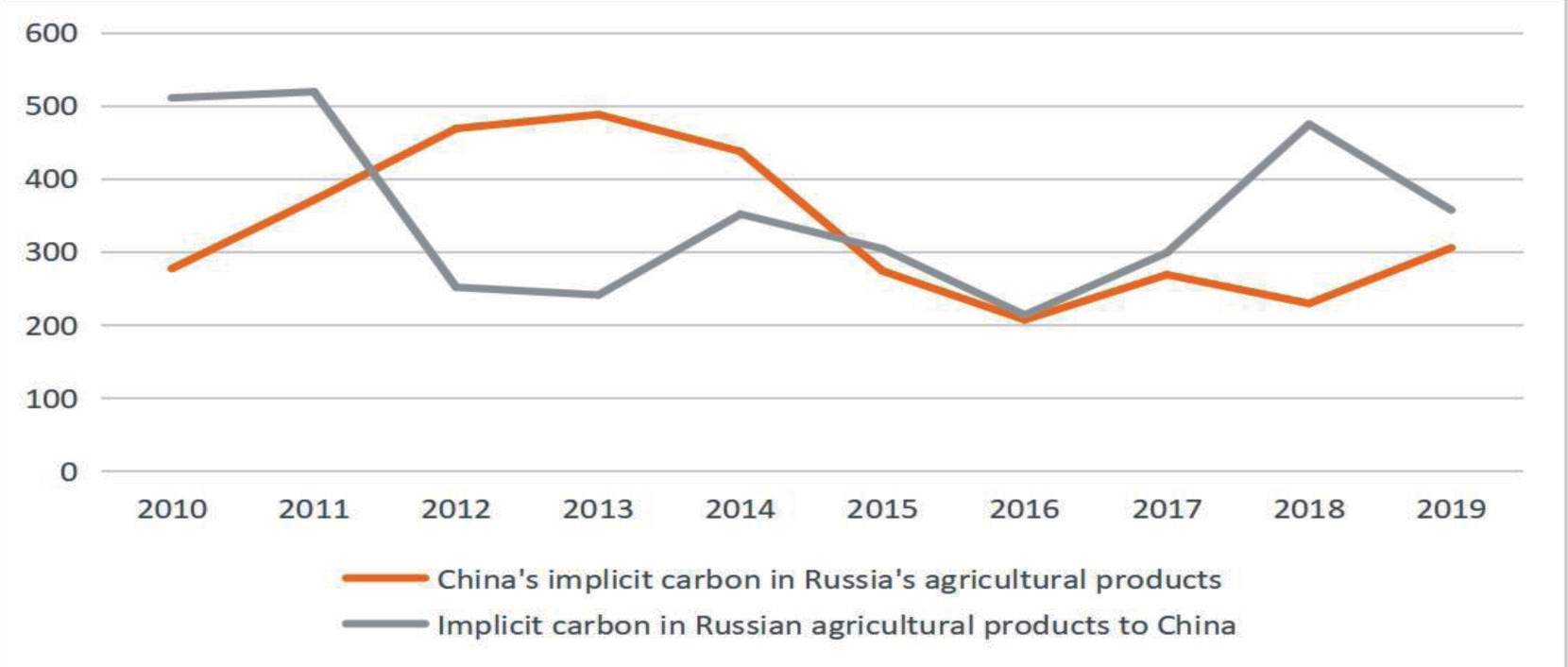
Figure 1 illustrates the fluctuation in China-Russia agricultural trade’s total embodied carbon volume (2009-2019). China’s embodied carbon emissions from agricultural exports to Russia varied between 2.06 million and 4.88 million tons. Emissions increased from 2009 to 2013, declined to 2.07 million tons from 2013 to 2016, and fluctuated after that, reaching 3.05 million tons in 2019 (a 24.9% YoY increase). Russia’s emissions to China ranged from 2.4 million to 5.19 million tons, peaking in 2011. Stability followed until a sharp increase to 4.74 million tons in 2018 (a 58.8% YoY rise), emphasizing the need for an improved trade environment.
Table 3.
Various energy consumption coefficients
Table 4.
Direct carbon emission coefficient (in tons)
Classification and Analysis of Embodied Carbon Emissions from Agricultural Products Trade Between China and Russia
Table 5 shows the changes in embodied carbon emissions of the three categories of agricultural products exported from China and Russia in 2009-2019, and through the statistical values in the table, we can intuitively find that in the trade of the three categories of agricultural products, due to the characteristics of the production of the products, the C3 category of agricultural products produces the most embodied carbon emissions, followed by the C1 category of traditional agricultural products, and the C2 category of farm products, the natural gas, gasoline and other energy consumption inputs in the production process, C2 agrarian products, in the production process of natural gas, gasoline, coal and other energy consumption is low, resulting in its own direct carbon emission coefficient is low, as well as in the trade volume and the scale of trade value added generated by China and Russia accounted for a small proportion, so this category of agricultural products in the three categories of agricultural products of the lowest embodied carbon emissions.
Summary Analysis
The analysis of embodied carbon emissions from China-Russia agricultural trade reveals distinctive trends. China’s exports to Russia initially increase, then decrease, while Russia’s exports to China show a reduction Source: Based on the embodied carbon emissions formula. followed by an increase. Overall, Russian exports exhibit slightly higher carbon emissions.
Table 5.
Embodied carbon emissions from China-Russia classified agricultural exports (in tons)
In sub-sectors, C3 plant and timber products, with higher energy consumption, lead to significant carbon emissions, topping the list. Traditional C1 agrarian products, despite high trade turnover, rank second due to lower energy consumption. C2 products follow with minor carbon emissions.
Trends in embodied carbon correlate with shifts in overall trade volume, influenced by key events like the 2008 financial crisis, Russia’s WTO accession in 2012, the “Belt and Road” initiative in 2013, Western sanctions in 2014, and U.S.-China trade relations in 2018. Critical change nodes include the 2008 financial crisis, Russia’s WTO accession in 2012, the “Belt and Road” initiative in 2013, Western sanctions in 2014, U.S.-China trade friction in 2018, and trade fluctuations from the Russian-Ukrainian conflict in 2022. Further Analysis: Decomposition Analysis of Factors
Affecting Embodied Carbon Emissions from China-Russia Agricultural Trade
Analysis of Implicit Carbon Decomposition in China’s Classified Agricultural Exports to Russia
(1) Trade scale: C1 product emissions from China to Russia initially decrease then increase, closely tied to trade scale changes. C2 emissions follow the same pattern as trade scales, decreasing with reduced trade. C3 emissions correlate positively with scale but decrease from 2014 to 2018 as the scale drops. However, C3’s positive impact on emissions diminishes as the scale decreases.
(2) Structural effects: C1’s structural changes increased emissions after 2017. C2’s primarily positive structural effect increases emissions, turning negative
after 2018. C3’s structural effect initially promotes emissions, then turns negative, driving reduction.
(3) Intensity effect: C1’s low energy efficiency increased emissions from 2014-2018, improving in 2019. C2 and C3 show consistently harmful intensity effects from 2010-2019, indicating that progress in energy efficiency drives emission reduction. Table 6 shows the specific results.
Analysis of Implicit Carbon Decomposition in Russia’s Classified Agricultural Exports to China
(1) C1 product emissions to China from Russia had varying scale effects, positive in 2010-2011 and 2017- 2018 but negative in 2019. C2 emissions had minimal and steady scale effects, peaking in 2017. C3 scale effects fluctuated, causing emission growth in 2010- 2011 and 2017-2018 but a decline in 2019.
(2) C1 structural effects were adverse in 2010-2015, turning positive in 2019. C2 had a positive structural effect in 2010-2015, turning negative in 2017-2019, aligning with emission decline. C3 showed positive structural effects in 2010-2015, turning negative in 2017-2019, consistent with emission reduction. The structural effect of C3 was positive in 2010-2016, turning significantly negative in 2017-2018, especially in 2018, and becoming positive again in 2019.
(3) C1 intensity effects were adverse in 2010-2014, turning positive after 2015, leading to increased emissions. Improved energy efficiency in 2019 resulted in a negative intensity effect and emission reduction. C2 consistently had a negative intensity effect, significantly reducing emissions, especially in 2018-2019. C3 had a negative intensity effect in 2011- 2013, turning positive in 2014-2018, but became negative again in 2019, the main factor in emission reduction. Table 7 shows the specific results.
Table 6.
Results of embodied carbon decomposition of China’s exports of three types of agricultural products to Russia (in tons)
Table 7.
Results of embodied carbon decomposition of Russian exports of three types of agricultural products to China (in tons)
Conclusions
Utilizing input-output data, a multi-regional model computes carbon emission coefficients, trade value-added, and embodied carbon emissions for three China-Russia agricultural product categories (C1, C2, C3) from 2009 to 2019. Findings reveal: (1) C3 has the highest carbon coefficients, followed by C1 and C2. (2) Despite high carbon coefficients for C3, Russian agricultural exports to China surpass China’s in value-added, with C1 leading, followed by C2 and C3. (3) Russia’s embodied carbon emissions to China exceed China’s to Russia, showing a declining trend for China and fluctuations followed by an increase for Russia; C3 products contribute the highest, followed by C1 and C2 with the lowest emissions.
Employing an LMDI index decomposition model from 2010 to 2019, influencing factors, including trade scale, structure, and carbon emission intensity, are examined. Results indicate: (1) Export scale is the primary factor increasing embodied carbon emissions for both countries, with structural effects playing a secondary role for China and intensity effects being the smallest. Russia exhibits intensity effects as the second-most significant factor.
(2) By industry, the intensity effect minimally promotes embodied carbon emissions for C1 products in both countries, while mainly restraining emissions for the other categories. Structural effects shift from restraint to promotion in the export trade of all three categories. Below are some policy recommendations:
Mitigating the scale effect is key to reducing embodied carbon in Sino-Russian agricultural trade. Instead of cutting trade scale, prioritize carbon emission reduction. For low-carbon trade, Chinese exporters should enhance energy efficiency, embrace clean energy, and receive government support. Global knowledge transfer in clean energy technologies is crucial.
To tackle rising carbon emissions from expanding trade, focus on agricultural decarbonization. Implement low-carbon technologies, raise awareness, and support government-led initiatives for sustainable practices in China.
For reduced embodied carbon in China’s agricultural exports to Russia, improve the trade structure. Diversify markets, leverage opportunities like RCEP, FTA, and “Belt and Road”, and enhance trade infrastructure for stability.
Fostering a sustainable, low-carbon model requires policy alignment, adoption of international emission standards, and refined carbon accounting. Expanding Sino-Russian agricultural trade is vital amid the Russia-Ukraine conflict for stability and effective carbon management.
Although this paper provides a detailed empirical analysis of the embodied carbon in Sino-Russian trade in agricultural products, the years studied are relatively limited due to data constraints, and future studies can further increase the sample size.