Introduction

Environmental problems refer to the decline in the sustainability of the air, primarily manifested through the pollution of air, water, food sources, and ecosystems. The primary contributor to this degradation is the release of carbon emissions from agricultural practices, livestock activities, and industrial processes. The agricultural industry contributes significantly to the global economy, providing sustenance to people and playing a vital role in alleviating severe poverty and fostering rural development worldwide. Therefore, the growth of the agricultural industry holds paramount importance on a global scale. It is projected that by 2050, this sector will be instrumental in feeding a population of 9.7 billion people worldwide [1-3]. Agriculture’s growth is two to four times more effective in generating income for the world’s impoverished compared to growth in other sectors of the global economy. In 2016, it was estimated that the agriculture sector employed 65% of the workforce [4]. The correlation between agriculture and economic growth is profound and has far-reaching implications for the global economy. The contribution of the agricultural sector to the global GDP remained at 4% from 2000 to 2020. However, in some emerging economies, this contribution is approaching 25%. Notably, between 2000 and 2020, the agriculture sector’s value-added increased by 68%, equating to approximately USD 4.4 trillion [4].

China possesses a substantial agricultural sector, utilizing 7% of the world’s arable land to produce grain for 22% of the global population [5]. China has employed intensive agricultural practices with heightened inputs for decades to ensure robust crop yields, resulting in agricultural greenhouse gas emissions accounting for 17% of total emissions. However, efforts to promote low-carbon technologies have gained traction in recent years [6]. To capitalize on these opportunities, it becomes crucial to conduct carbon footprint assessments for various agricultural ecosystems in China.

As China pursues industrialization and modern technologies for economic advancement, the agricultural sector not only provides sustenance but also fuels agro-based industries. While it holds potential to safeguard the environment, the shift from traditional agriculture to the industrial sector has led to environmental decline [7, 8]. Despite its global significance, the agricultural sector confronts ongoing challenges such as meeting the demand for high-quality food, efficient allocation of natural resources, biodiversity conservation, and improving societal welfare, especially in developing countries. Climate change emerges as a critical concern, impacting agricultural revenue and productivity, particularly in climate-sensitive regions like China. Surprisingly, forestry, land use, and agriculture contribute to 25% of greenhouse gas emissions. Addressing climate change challenges requires adaptation strategies [9].

The cornerstone of agroecology is the agricultural ecosystem, comprising both biotic and abiotic elements interacting with each other and the environment. Agroecological sustainability aims to provide healthy, safe, and balanced food while generating social value, even as practices such as deforestation and converting forest and orchard land to arable land have altered agricultural ecology. Novel resource utilization strategies have increased food production for the expanding global population, but they have also led to lasting environmental repercussions, including insect invasions and soil fertility decline [10, 11]. Climate change poses a substantial threat to the existing monoculture agricultural system. Although the agricultural ecosystem shows resilience to climate change, reducing the carbon footprint based on agricultural ecosystems requires efficient energy use and climate-resilient agricultural practices. Evaluating the ecological footprint of the agricultural ecosystem is of paramount importance, reflecting a country’s assimilation capacity on a broad scale while also showcasing the intensity of greenhouse gases, energy, inputs and outputs, and energy consumption at a local level [12]. Human activity has led to environmental deterioration, as evidenced by rising temperatures, erratic climate patterns, and continuous ozone depletion. Numerous studies, including those by [13-15] have highlighted the connection between agricultural expansion, operations, activities, and environmental degradation in various nations. The increasing demands on food and the rapid population increase are causing an acceleration of human effects on the land and other natural resources. This study is important because it clarifies how pressure from growing agricultural intensity affects land resources as well as the environment as a whole. Because of these concerns, the agricultural sector is given significant importance in both economic and environmental policies.

The complex links that agriculture has with natural resources and the environment make it difficult and incomplete to attribute specific environmental effects to it. Agricultural productivity depends on both quantity and quality, even though it consumes a large amount of land and water. Among agriculture’s negative environmental effects are decreased planned biodiversity, untreated animal feces, water pollution, and soil erosion. Studying how all forms of agriculture affect the environment is vital since there is a contextual gap in the literature, with past research focusing on the effects of rural and urban agriculture. Despite the limited documented research in the literature, the existing gap underscores the need for fresh exploration into the impact of agricultural systems on the environmental footprint. This study aims to examine the influence of agricultural ecosystems on environmental footprints in China. The results of this research promise insights into ecologically sound agriculture and a sustainable China. Additionally, the study employs the ARDL approach to analyze both exogenous and endogenous factors in the short and long term within the Chinese context.

The structure of the research is as follows: Section 2 provides a literature review. Section 3 outlines the methodology, while Section 4 presents the results and discussion. Section 5 concludes the study with policy recommendations.

Review of Literature

Globally, rising demand for agricultural goods frequently runs counter to the goal of environmental protection [16]. This is especially true in China’s agricultural sector. The successful attainment of food and nutrition security has led to significant environmental damage, impacting the landscape, water, nutrients, and biodiversity. Agriculture-related pollution sources include agrochemical misuse or overuse, improperly managed sewage from livestock farming, contamination from irrigation water, and so on. According to Norse and Ju [17], the economic loss due to environmental damage, including such adverse effects on the sustainability of food manufacturing and human health, ranges from 7% to 10% of China’s agricultural GDP. For example, the researchers identify nitrogenous fertilizer overuse as a major cause of economic loss.

The association between agricultural activity and environmental contamination and deterioration has been studied by earlier academics. The relationship between agricultural practices and carbon emissions was investigated by Yu and Wu [18]. The study’s findings showed that agriculture is the primary contributor to pollution and environmental deterioration. Long et al. [19] carried out a comparable investigation in China. It was discovered that China’s agriculture significantly affects carbon emissions. Furthermore, while innovation within the nation reduces carbon emissions, foreign direct investment raises them. In a similar vein, Chandio et al. [20] investigated how energy, growth, and environmental quality relate to the agricultural industry. The study’s analysis came to the conclusion that growth and energy use had a favorable influence on carbon emissions. These findings suggest that increasing agricultural production and energy use degrade the ecosystem.

The relationship between Saudi Arabia’s agricultural development and carbon emissions was studied by [21]. According to the findings of their research, the country’s carbon emissions are negatively impacted by the expansion of agriculture. Additionally, their findings disagree with those of [22]. They examined the impact of carbon emissions on the current Indian agricultural ecosystem from 1990 to 2014. Their research showed that agricultural practices and activities are a significant contributor to pollution and environmental deterioration in India. They also confirmed a one-way causal association between CO₂ emissions and agricultural technology, insecticides, animals, and animal waste used in the agricultural environment. However, a two-way causal link between carbon emissions and biomass production from burned agricultural leftovers was discovered. These findings reinforced the notion that the agricultural ecosystems of the United States had a considerable influence on CO₂ emissions. Furthermore, other research, such as Cox et al. [23], found comparable results. Using time-series data from Portugal, the author examined the link between agricultural productivity and CO₂ emissions. The study’s findings revealed that factors such as land productivity, labor employed in agricultural production, and agricultural raw material exports all contribute to increased carbon emissions. These data showed that agricultural activities resulted in more pollution and environmental degradation.

In addition to the research indicated above, Sarkodie and Owusu [25] used time series data for Ghana from 1961 to 2012 to explore the association between agricultural and livestock output and carbon dioxide emissions. It was discovered that the nation’s crop and animal industries produce carbon dioxide emissions. Ravindra et al. supported these findings (2019). From 2003–2004 to 2016–17, they looked at the connection between agricultural crop wastes and air pollution in India. The results of the studies [26, 27] were supported by the study’s analysis. Similar to this, researchers [28] examined the relationship between Tunisia’s agricultural and economic development and carbon dioxide emissions. They came to the conclusion that agriculture increases carbon emissions. To cut carbon emissions and boost the sector’s growth, they recommended using renewable energy in agriculture.

The amount of GHG emissions caused by agricultural management practices such as tillage, inorganic fertilization, and cultivation [29], pesticides, minoring, waste disposal, composting, biochar addition, and crop photosynthetic activity capacity are all linked to the carbon footprints of agricultural inventions. As a result, sustainable agriculture approaches must be studied in order to address these concerns. Similar to this, Environmental Kuznets Curves (EKC) were investigated by Liu et al. [30] in panel data cases including 4 ASEAN nations. They claimed that in the cases of 4 ASEAN nations, EKC is invalid. Rafiq et al. [31], on the other hand, used panel data from 53 counties to illustrate the validity of the EKC hypothesis in the area of agriculture. In a related study, Ridzuan et al. [32] studied the effects of agriculture, renewable energy, and economic activity on emissions of CO₂ in Malaysia from 1978 to 2016. According to their findings, agriculture and fishery have a negative influence on the country’s carbon emissions, while livestock has a positive benefit.

The ecology and biological literatures account for a large portion of the literature cited in the current section. This is partly caused by the inherent intensification dynamics, which are fascinating in and of themselves. More focus from social scientists can guarantee that farmers’ choices are considered in these investigations and that causation is treated properly. Of course, achieving this goal necessitates exogenous change in intensity, which is uncommon and reduces the possibility of doing in-depth causation analysis in earlier investigations for the environmental impacts of agricultural practices in China, which this study aims to perform.

Econometric Model and Methodology

The study looked at the relationship between China’s agro-ecosystem and its environmental footprints, using data from a variety of sources from 1990 to 2020. Appendix 1 covers all of the variables and data sources used in the research. The dependent variable is the environmental footprint, which is expressed as a global million-hectare footprint. This variable data was obtained from the Global Footprint Network, which supports the science of sustainability (GFN, 2021). The environmental footprint represents the restrictions and deterioration of the environment caused by human actions and operations. Farmland, cultivated land, greenhouse gas emissions, forest, fishery, and livestock all contribute to the environmental footprint [33, 34]. There are five explanatory variables. These factors represent China’s agro ecosystem as a whole. The environmental footprint has a strong correlation with the inclusion of the entire agro ecosystem. These variables were chosen based on the literature of earlier research projects’ theoretical basis. For instance, previous studies have shown that factors such as energy consumption, rainfall, temperature, livestock and stock, fertilizer, nutrients, biomass burned dry matter, and employment in agriculture have an impact on environmental quality [35-37]. Data for agricultural land and employment factors were gathered on 1000 Hectors and 1000 individuals, respectively. Fertilizer by nutrient was expressed in tons. Statistics from the Food and Agriculture Organization were used to create these variables (FAO, 2021).

The link between an agro-ecosystem and its environmental footprint was determined using the time-series model indicated in equation 1. The logarithmic function was used to record the results of the investigation. Other benefits of using the logarithmic function model include decreasing the data, reducing its sharpness, boosting its dependability, and standardizing the data. The log-transformation co-efficient is viewed as a direct elasticity in the model [38, 39].

Here, β provides the parameter, t displays the time period under analysis, and ε represents the regression model’s error term in Equation 1. Additionally, the LnEFP displays environmental footprint, the LnAGL denotes agricultural land, the LnAEM denotes agricultural employment, the LnEN denotes agricultural energy usage, the LnFRN denotes nutrient-based fertilizer, and the LnLS denotes livestock number.

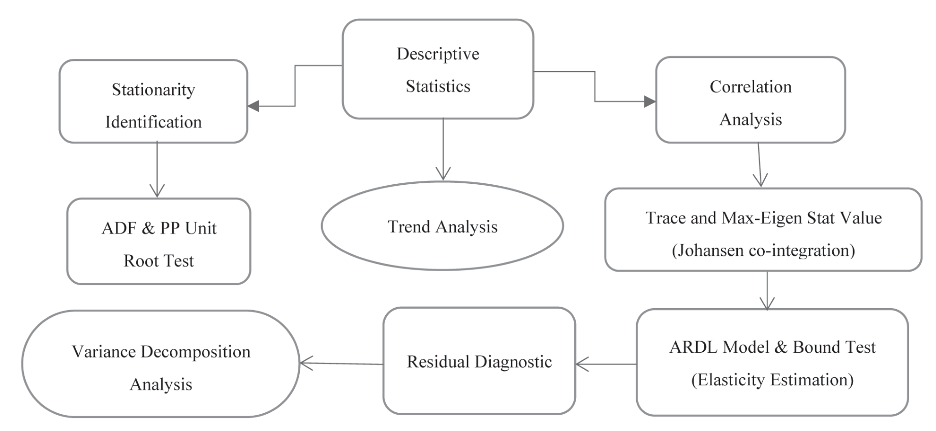
Figure 1 depicts the flow chart for the research process. We began by doing inferential and descriptive statistics, correlation, and trends on the study in accordance with this flow chart. After completing the fundamental task, we ran a stationary test, also known as the unit root test. We picked our model for the investigation based on the unit root results. The Johansen cointegration test was developed to look into the long-term relationship between an agro-ecosystem and its environmental impact. The trace and Max-Eigenvalue tests comprise the Johansen test [40]. The Max-Eigenvalue test findings would be evaluated if the results were not similar. Because Max-Eigenvalue gives more robust and reliable findings (41):

Equations 2 and 3 state that K denotes sample size and V denotes cointegration vectors. The λ value of them is ordered. The symbol π denotes the coefficient of the eigenvalue matrix. The alternative is assessed against the null hypothesis using the Johansen trace test (V). This indicates that H₀: rank π ≤ V against H₁: rank π > V. Here, the Johansen MaxEigen value (V + 1) is used to compare the statements H0: rank π ≤ V against H1: rank π = V + 1.

We employ the ARDL strategy in the subsequent model in this work. Prior to doing this model and bound test, the long-run connection was investigated using the Pesaran et al. (2001) method. There are several properties of the ARDL model, such as the fact that it may be performed regardless of the integrated order I(0) or I(1), and that it provides direct elasticities of the variables. This method is, however, quite sensitive to the lag-length requirements. As a result, PESARAN et al. decided to calculate the lag-length order using AIC criterion (2001). The econometric specification for the ARDL model in this work is as follows.

Fig. 1.

Flow chart of the research process

In Equation 4, the differentiation operator is denoted by ∆, and a and c denote the short-run and long-run parameters, respectively. While μt stands for the error term, a residual term that is serially independent. Furthermore, the estimate of diagnostic statistics was used to econometrically cross-check this model. The diagnostic data imply that the study’s ARDL model specification is genuine, normal, valid, and accurate.

Results and Discussion

The descriptive statistics and correlation for all variables considered in the study are shown in Table 1. With the exception of agricultural land, all independent variables exhibit a positive and significant correlation with environmental footprints. The use of descriptive statistics shows that all of the variables’ characteristics are consistent, ordinary, and balanced. This shows that there are no outliers in the data.

This study starts a formal time series analysis after conducting the preliminary analysis. We started by using the unit root test. We utilized PP and ADF tests to analyze the unit root integration. Table 2 displays the results of the ADF and PP tests. These findings demonstrated that every variable is integrated to order one. The study’s subsequent models may be immediately applied as a result of the unit root. In order to assess the long-term link between an agro-ecosystem and ecological footprint in the example of China using Johansen co-integration, we first base our analysis on the integrated order.

The Johansen test results are shown in Table 3. The Johansen cointegration test consists of two additional tests. First is the max-Eigen value, and second is the trace statistics. Whereas the Trace test has five co-integrated vectors, the Max-Eigen value has four. These results showed a long-term relationship between environmental footprints and the agro ecosystem.

In this work, the ARDL approach examined the agro ecosystem’s short-run and long-term elasticity on environmental footprint. To begin, we investigate the bound test approach for ARDL in order to run the ARDL model. This test has two features: lag length sensitivity and the integrated order of the variables in the data. Concerning the Bound test ARDL model, these concerns were allayed, and the ARDL model performed well. As a consequence, the AIC criteria were chosen since they had the lowest value of all the criteria stated in Table 4. ARDL is the best framework with lag-length (1, 1, 0, 0, 0, 0, 0, and 1).

The F statistics value is between the upper and lower bound values in Table 5, indicating that the ARDL bound test is valid. According to the bound test’s validity, the ARDL model is dynamically stable, and the long-run relationship is valid.

Table 6 depicts the ARDL relationship between the agro-ecosystem and the environmental impacts in the short and long run. The ARDL model’s co-integrated form demonstrates how an agro-ecosystem’s ecological footprint changes over time. Additionally, since all of the variables are already taken into account in logarithmic form, all of the coefficients are considered to have direct elasticity. Based on the findings shown in Table 6, the ARDL’s short-run model predicts that a 1% increase in China’s agricultural area would result in a 0.19% rise in the nation’s ecological footprint. However, over time, this quantity (0.75%) seems a little high. Furthermore, agriculture’s energy, fertilizer, and employment practices all have a significant immediate and long-run impact on the ecological footprint. Based on this, China’s environmental footprints grow by 0.56%, 0.35%, and 0.54% for every 1% increase in employment, energy consumption, and fertilizer use in agriculture. The ARDL model is inherently stable since the co-integration results in Table 5 show a highly negative coefficient. This suggests that all of the model’s variables move together and dynamically.

Several diagnostic statistics were run in order to assess the ARDL model’s validity, credibility, and stability. The findings are displayed in Table 7 for your perusal. These findings demonstrated that the ARDL model is genuine, stable, normal, and compatible with model specification, according to the χ2 RESET, CUSUM, and JB tests. Furthermore, the model’s predictions for autocorrelation and heteroscedasticity issues are supported by χ2 LM and χ2 ARCH. This suggests that the ARDL model is immune to these problems.

The AR root model was used to analyze the stability state of the VAR model. According to the AR root diagram model, the model is deemed stable if the inverse roots of the AR characteristic polynomial are less than 1.

Agricultural activities contribute significantly to global greenhouse gas (GHG) emissions. They account for 17% of total GHG emissions in China, and there are methods that may be used to minimize GHG emissions, such as correct agro-chemical application, enhancing ruminant nutrition, and intermittent irrigation of rice paddy areas [42, 43]. Nitrogenous fertilizer misuse not only adds to soil, water, and air pollution, but it is also a source of greenhouse gas emissions: in China, 13.5 tons of CO₂ – equivalent is generated for every ton of fertilizer made and consumed [43]. China’s initiative is critical for decreasing N-related greenhouse gas emissions since it is the world’s largest consumer and producer of N fertilizer.

Generally, there are links between agricultural sustainability and ecological sustainability. A major factor in agricultural output, which is necessary for humans, is the ecological system. However, this enormous contribution to agriculture leads to a worsening of the natural system with the growing population [44-46]. Ecosystem services are among the benefits of the ecological system. Land usage affects agricultural activities. As a result, ecosystem services are significantly impacted by changes in the land caused by agricultural operations [47, 48]. On the one hand, ecosystems promote agriculture yield via improved crop pollination and reduce the likelihood of frequent floods through forestation. On the other hand, agricultural practices affect ecosystem services in both good and bad ways [49-51]. However, the major focus of this study is on the detrimental effects of agricultural activities on natural systems. The study’s findings revealed that China’s agro-ecosystem activities—such as the use of agricultural land and labor, energy consumption, and fertilizer application—increase the country’s ecological footprint. It is standard practice for these agricultural practices to increase crop output at the expense of the environment. Additionally, agricultural residue burning is a practice that requires prompt government intervention in order to stop the environment’s decline.

Conclusion and Policy Implications

This study focuses on the relationship between China’s agro-ecosystem and ecological impact. Modern econometric methods are used in the study, including Johansen and ARDL approaches. ADF and PP tests were run before undertaking formal analysis in order to prevent stationarity issues. The Johansen experiments’ findings showed how an agri-ecosystem’s sustainability and environmental impact can change over time. According to the ARDL model’s short- and long-run elasticity results, there is a positive association between agricultural land, employment, energy usage, and fertilizer use in agriculture. Alternately, the diagnostics and inverse AR tests demonstrated that the ARDL model’s functional shape and stability are proper.

The findings indicate that agricultural practices in China should be altered in the future to reduce environmental impacts. Additionally, the article demonstrates that the Chinese government should pay closer attention to pollution levels and considers the agriculture sector to be one of the primary sources of pollution. As a policy recommendation, the government should support initiatives such as organic farming via the use of new ecologically friendly technology, as well as the prudent use of chemical fertilizers and pesticides, in order to lower the country’s pollution levels and environmental footprints. In order to minimize energy consumption, greater emphasis should be placed on employing energy-saving lighting and irrigation technologies on farmlands. Additionally, public knowledge of air pollution generated by various industries should be increased, since insufficient education and disregarding possible pollution dangers might contribute to pollution.

As a result of the facts presented above, several policy implications emerged from this paper. This study showed that, in an effort to increase output and productivity, agricultural production farming damages the environment and natural resources. At many C from different sectors are not always coherent and can even be at odds with one another. Public policy can also have unanticipated consequences, especially when it affects the behavioral incentives of certain stakeholders. Coherent integration of policies into the system takes more planning and work. In order to boost agricultural output, more chemicals and fertilizers are required. Therefore, organic fertilizer must be utilized rather than inorganic fertilizer. Raising cattle needs special care in order to produce more manure, in addition to more meat, milk, etc. To decrease the amount of high energy usage in agriculture, zero tillage should be adopted. The country should be made aware of the breadth and idea of green products, and policies should be put in place to implement contemporary low-carbon emission technologies. This study will assist academics, policymakers, researchers, and planners in developing a clear strategy and vision for supplying sustainable food and environmental conditions.

Sustainable agriculture requires the preservation of natural resources. Future generations will struggle as a result of excessive activity that is carried out without allowing natural resources to replenish themselves. This is the main reason why it is important that the goals on this topic are well-defined and unambiguous, and that unsustainable agriculture practices are discouraged. Governments and non-governmental organizations should provide controls and training to prevent activities like over-irrigation of the soil, overuse of fertilizers, and improper spraying that could damage the ecosystem. A sustainable agriculture database should be created, along with the technological, social, and financial data bank applications that are required. This study’s shortcomings include its inability to address the significance of resource reallocation in determining land use outcomes, the energy consumption of the agriculture sector, and the underrepresentation of agricultural workers in both the literature and this study. It would also be beneficial to investigate the ways in which other market failures, like a lack of knowledge or a poorly defined agricultural output, influence which outcomes end up winning out.