

Introduction
Agriculture is a fundamental industry that underpins the construction and advancement of the national economy. Since the implementation of reform and opening-up policy, China’s agricultural production has experienced rapid growth, resulting in a gradual increase in food output and significant expansion of agricultural economic output. Nevertheless, agricultural development continues to face profound challenges. On the one hand, agriculture faces major challenges to its long-term sustainability: over-development of agricultural resources, overuse of agricultural inputs, over-development of groundwater, and the overlapping of internal and external sources of pollution in agriculture [1]. On the other hand, the degradation of agricultural ecosystems is obvious; the institutional mechanisms for water and soil resource management and ecological compensation are not sound; the constraints on water and soil resources are becoming increasingly tense, and the promotion of sustainable development in agriculture has become urgent [2-5]. The No. 1 Document of the Central Government in 2023 further emphasized a series of important initiatives to promote green development in agriculture. AEE is an important indicator for measuring the green and sustainable development of agriculture, and scientific evaluation of AEE is conducive to accurately assessing the true level of agricultural ecosystems and realizing the efficient use of agricultural resources. The key to greening agriculture in the new stage of development lies in improving AEE. Existing studies show that China's agricultural carbon emissions account for 16 to 17% of national carbon emissions, much higher than the international average level [6]. In the context of "double carbon”, i.e., peak its carbon dioxide emissions by 2030 and achieve carbon neutrality by 2060, it is far from enough to evaluate the efficiency of agricultural production only from the perspective of economic efficiency, and there is an urgent need to incorporate agricultural carbon emissions into the evaluation system of AEE, to truly reflect the development of agriculture.
Current research on AEE focuses on three main areas:(1) Construction of AEE evaluation index system, which usually includes labor, land, capital, fertilizer, pesticide, agricultural film, draft animal, machinery, etc. into the input indicators [7-9], classification of output indicators into desired and non-desired outputs, with gross agricultural output included in desired outputs, agricultural surface pollution and carbon emissions [10].
(2) In terms of evaluation methods, scholars mainly use data envelopment analysis (DEA) and its derived models [11, 12] and non-expected SBM models [13], stochastic frontier analysis (SFA) [14], life cycle assessment (LCA), and other evaluation methods. Some scholars have also integrated LCA and DEA methods for comprehensive measurement [14, 15], and analyzed the spatial and temporal evolution of AEE using Malmquist index [16], spatial Durbin model [17], and spatial Markov chain [18] to analyze the spatial and temporal evolution of AEE. Among them, the super-efficient SBM model with non-expected output has unique advantages in measuring AEE, which can effectively avoid the bias caused by radial and angular metrics, and consider the influence of non-expected output factors, which better reflects the nature of the efficiency evaluation, and has been widely cited by the academic community.(3) In terms of the factors affecting AEE, scholars have used the Tobit model [19], the STIRPAT model [20], and geographical detector [21] to analyze the impact of elements such as the urbanization rate [19], agricultural science and technology inputs [22], resource endowments [23] and low-carbon pilot policy [24] on the AEE. The green and low-carbon development of agriculture is a systematic project, and the coordinated development among the constituent elements is the key. There are certain spatial aggregation and differentiation phenomena among regions, and the roles of the elements in different periods are also different. However, the existing research have considered the spatial dimension more, and have not considered the time factor sufficiently. Therefore, it is necessary to include the time dimension and adopt the GTWR model in order to understand the spatial and temporal patterns of AEE scientifically.
Fujian Province, located on the southeast coast of China, is a hilly region with scarce arable land resources, resulting in an uneven spatial distribution of agricultural production resources across the province [25]. As a representative of a hilly region, affected by natural factors, it is more difficult to achieve large-scale and mechanized production in most areas of Fujian Province, resulting in the AEE of Fujian Province being prone to discrepancies and fluctuations [26, 27]. In addition, in 2014, Fujian Province became China's first ecological civilization demonstration area, which means that agroecological development will become an important way to achieve ecological civilization in Fujian [28]. Therefore, it is of great significance to conduct research on AEE in Fujian Province in order to effectively promote the development of AEE and complete the construction of ecological civilization pilot area. Consequently, this study incorporates the element of carbon into the evaluation system of AEE, and adopts the unexpected output SBM super-efficiency model to measure the value of AEE in Fujian Province from 2000 to 2020.On this basis, spatial autocorrelation analysis and spatio-temporal geographically weighted regression model (GTWR) were applied to further analyze the spatio-temporal dynamic characteristics and heterogeneity of AEE in Fujian Province, in order to provide decision-making references for the green transformation of agriculture and supply-side reforms in the context of the new period.
Material and Methods
Overview of the Study Area
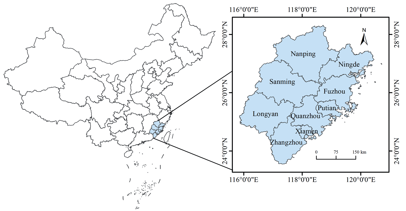
Fujian is located between latitudes 23◦33´ and 28◦20´ North and longitudes 115◦50´ and 120◦43´ East, crossing the central and southern subtropics, the north and Zhejiang as a neighbor, the northwest border with Jiangxi, the south border with Guangdong, and Taiwan is connected by water (Fig. 1). The total land area of Fujian Province is 121,800 square kilometers (including Kinmen County). Fujian Province is mountainous, with towering peaks, winding mountain ranges and rolling hills, known as “eight mountains, one water, one field”. Under the influence of monsoon, climatic disasters are frequent, but the topographical conditions, and the rain and heat conditions have created the characteristic agricultural production conditions in Fujian Province. In 2021, the added value of agriculture, forestry, animal husbandry and fisheries increased by 3.5%, the per capita disposable income of farmers increased by 8%, and the coverage rate of good agricultural seeds reached 98.5%. In 2021, the annual grain sowing area in Fujian Province was 12.526 million acres, with a total production of 5.064 million tons. To achieve sustainable agricultural development in Fujian Province, it is necessary to further coordinate the balance between agricultural economic development and environmental protection.
Research Methodology
System of Indicators
Based on the existing literature review [29-33], in combination with data availability and compatibility of statistical metrics, we constructed an AEE evaluation index system with land, fertilizers, pesticides, agricultural films, machinery, irrigation, labor, energy, and draught animal as input indicators. The index of the total output value of the agriculture, forestry and animal husbandry industry was taken as the desired output, while the amount of agricultural carbon emissions and the amount of agricultural surface source pollution were taken as undesired outputs (Table 1). The amount of agricultural pollution was calculated by the entropy method based on the amount of fertilizer waste, the amount of ineffective pesticide use, and the amount of agricultural film residue [6, 25, 34].
AEE is affected by many factors, with reference to the previous studies [19, 35-38] combined with the reality of agricultural development in Fujian Province and the availability of data, this study selected six influencing factors, namely, the urbanization rate, farmers’ income, mechanization, agricultural resources endowment, planting structure, and financial support.
Estimation of Agricultural Carbon Emissions
Based on existing literature regarding agricultural carbon emissions [39-42], this study mainly estimated agricultural carbon emissions from fertilizer, pesticide, agricultural plastic film, agricultural machinery, irrigation, diesel fuel consumption, ploughing, crop sowing, animal enteric fermentation, and manure management. The carbon sources and coefficients used in this paper were obtained from the research of Chen, Wang, and Huang et al. [25, 40, 42]. The estimation of carbon emissions was as follows:
Where C is the total agricultural carbon emission; Cit is the carbon emission of carbon source i in year t. Eit is the amount of carbon source i in the year t. And δi is the agricultural carbon emission factor for each carbon source i. This paper evaluated and calculated three types of carbon emissions (C, CH4, and N2O), and converted them to standard carbon based on the IPCC.
Table 1.
AEE evaluation index system.
Table 2.
Factors affecting AEE.
Super-Efficient SBM Modelling of Undesired Outputs
In addition to the desired outputs of agricultural, forestry, and livestock production, there are also undesired outputs in the agricultural production process. The SBM model, which is based on non-expected outputs, boasts clear advantages for managing the non-expected outputs of AEE. It is able to comprehensively consider the slack phenomenon of input factors. Additionally, the super-efficient SBM model addition eliminates the issue of multiple effective decision units that cannot be comparatively analysed. The model is constructed as [43]:
(2)
Where X denotes the AEE value. Assume that there are n decision-making units DMUs, each with inputs, desired outputs r1 and non-desired outputs r2; x, yd, and yu are elements in the input matrix, desired output matrix, and non-desired output matrix, respectively.
Spatial Autocorrelation Analysis
AEE varies across regions due to differences in available resources, agricultural economic development and other conditions. However, agricultural development in each region does not occur in isolation. The first law of geography posits that conditions such as geographical location impact not only the AEE of the region but also neighboring regions. In this study, the overall status of AEE in Fujian Province was investigated using global spatial autocorrelation analysis.
The degree of spatial autocorrelation in AEE was assessed using the Global Moran's I index which is in the range of [-1,1]. A positive spatial correlation is indicated by Moran's I>0, with a stronger spatial aggregation effect estimated as the values approach 1. When Moran's I is less than 0, there is negative spatial correlation and the closer the value approaches -1, the more notable the convergence displayed in the spatial distribution. A Moran's I value of 0 indicates that AEE is randomly distributed in space, with independent spatial object units. Global spatial autocorrelation is modelled as follows [44]:
Where I represents the Moran’s I index of AEE, wij is the spatial weight matrix; xi and xj denote the AEE of cities i and j respectively; x̅ is the average value of AEE for each city at the prefecture level.
In the actual distribution of spatial data, there is often the emergence of local area variable data due to the randomness of the data leading to the emergence of local instability, which requires the introduction of local spatial autocorrelation indices to evaluate the autocorrelation of the local area and reveal the spatial heterogeneity. In terms of spatial location, the Local Moran's I index is defined as [44]:
The statistics to be tested for the Local Moran’s index are as follows:
The types of local regional AEE aggregation can be classified into four categories based on the direction of Ii and Zi. where HH is the high AEE agglomeration area; LL is the regional low AEE spatial correlation area; HL is the regional high-low AEE spatial correlation area, which indicates that municipalities with higher AEE are surrounded by neighboring municipalities with lower AEE; and LH is the low - high AEE correlation area, which indicates that municipalities with lower regional ecological efficiencies are surrounded by neighboring municipalities with higher values [44].
GTWR Model
The spatio-temporal geographically weighted regression (GTWR) model adds the time factor to the geographically weighted regression (GWR) model. This effectively addresses spatio-temporal non-stationarity and can accurately estimate the factor parameters. The model is shown below [45]:
Where (μi, vi, ti) is the spatio-temporal coordinates of the ith sample unit; X and Y are the explanatory and interpreted variables, respectively; p is the number of explanatory variables; β0(μi, vi, ti) is the intercept term; βk(μi, vi, ti) is the estimated coefficient of the kth explanatory variable; and εi is the model residuals. The implementation of the GTWR model in this study is mainly based on the ArcGIS 10.5 software, and the GTWR plug-in produced by Huang et al. [46] is used to complete the calculation.
Data Collection and Processing
The research focuses on the AEE of nine cities in Fujian Province, with the selection of panel data from nine prefecture-level cities in Fujian Province between 2000 and 2020. The information was primarily sourced from the China Rural Statistical Yearbook, Fujian Statistical Yearbook and Fujian Province statistical yearbooks. Additionally, some data was gathered from the statistical bulletins on economic and social development published by various regions and local statistical bureaus each year. Any gaps in the data were filled using an interpolation method. The emission factors for carbon in fertilisers, pesticides, and agricultural films, amongst others, are obtained from the “Guidelines for the Preparation of China’s Provincial Greenhouse Gas Inventories.” These emission factors are informed by the research results of the IPCC and the Oak Ridge National Laboratory in the United States [10].
Results and Analyses
Regional Differences in AEE in Fujian Province
The super-efficient SBM model was employed with non-expected outputs to assess the indicator system, as detailed in Table 1. The results are presented in Table 2. Previous research led to the classification of the AEE of Fujian Province into five tiers: efficient (p≥1), high level (0.8≤p<1), medium-high level (0.6≤p<0.8), medium level (0.4≤p<0.6), and low level (p<0.4) [1]. The trend of AEE in Fujian Province is showing improvement, indicating that policy measures aimed at AEE have been effective, especially since the issuance of Fujian Province’s implementation opinions in 2015. The opinions aimed at accelerating the transformation of agricultural development modes, conserving and making efficient use of agricultural resources, effectively managing agricultural surface pollution, reducing the use of pesticides and chemical fertilizers to increase their efficiency, and resourcefully utilizing agricultural waste. Consequently, AEE has significantly increased. However, the maximum efficiency value remains low at 0. The development of AEE in Fujian Province can be broadly categorized into three developmental stages. The period between 2000 and 2007 experienced fluctuating growth, with AEE displaying significant decreases in 2002 and 2006. From 2008 to 2015, AEE improved but at a slow pace. The phase between 2016 and 2020 presents a rapid upswing, particularly in Longyan, Putian, and Sanming. The growth of AEE is striking, including Longyan, which achieved significant progress between 2012 and 2014 with an AEE value growth of 0.310. Although there was a decline in 2015, Longyan has reached the effective level from 2016 to date.
Table 3.
AEE in Fujian Province, 2000-2020.
A comparison of the AEE values of nine cities in Fujian Province reveals significant regional differences. Xiamen stands out with an average AEE value of 1.056, due to the city's commitment to efficient and specialized agricultural practices. This is evidenced by strong and continuous investments in agricultural technology and ecology-based sustainable production methods over the years. Fuzhou has the lowest efficiency value at only 0.226, which represents a significant discrepancy. Quanzhou and Fuzhou have consistently demonstrated low efficiency levels for several years. This illustrates a clear polarization of AEE in Fujian Province.
Analysis of the Causes of Agro-Ecological Inefficiency
Table 4 presents the values of redundant variables for input and output indicators for every city in Fujian Province during 2020. The primary reason for the loss of AEE in Fuzhou and Quanzhou is the significant redundancy of agricultural factor inputs and undesirable outputs. From the perspective of agricultural factor inputs, Fuzhou and Quanzhou have different degrees of redundancy in each of the factors of land, fertilizers, pesticides, agricultural films, machinery, irrigation, labor, energy and draft animal. This indicates that there is an imbalance in the scale and structure of the inputs of agricultural factor inputs and other resources in the two cities, which has resulted in the inability to make full use of the resources of agricultural production resources. In terms of output, both regions have large excesses of agricultural carbon emissions and agricultural surface pollution, with Fuzhou having a more significant excess of agricultural carbon emissions and Quanzhou having a more significant excess of agricultural surface pollution output.
Spatial Correlation of AEE in Fujian Province
Global Spatial Autocorrelation Analysis of AEE
Based on the principles of spatial econometrics, the global autocorrelation Moran' I index of AEE and its Z-statistic test value and significance level P-value were calculated, and the results are shown in Table 5. The global autocorrelation Moran’ I indexes of AEE in Fujian Province from 2000 to 2021 are all negative, indicating that areas with high or low levels of AEE in Fujian Province are less likely to be spatially clustered. The global Moran’ I index was the smallest in 2015 at -0.455, with values closer to -1 indicating a more pronounced negative spatial correlation. The Moran’ I index is highest in 2000 at -0.112, the closer to 0 the more random the spatial distribution is in that year. The test for the Moran’ I index fails in all years, which may be related to the overall sample size, but the overall results suggest that the AEE in Fujian Province has mainly a random spatial pattern. Although the spatial correlation is not significant, Moran’ I has the characteristic of decreasing year by year, showing a spatial pattern of overall random distribution and possible aggregation at a small scale, which requires further local spatial autocorrelation analysis.
Table 4.
Decomposition of the causes of agricultural ecological inefficiency in Fujian Province in 2020.
Table 5.
Global autocorrelation index of AEE in Fujian Province.
Analysis of Local Spatial Autocorrelation in AEE
In order to more clearly show the spatial agglomeration characteristics of certain areas, key years were selected and LISA agglomeration maps were drawn (Fig. 1). The results show that (1) the L-L agglomeration area only appeared in 2000 in Ningde, the reason is that the city's topographic conditions, natural climate conditions hinder the intensive use of agricultural resources, but with the recent years of the development of agricultural modernization in the region and support for ecological production technology, Ningde, AEE began to improve no longer appear L-L agglomeration.(2) The L-H agglomeration is distributed in Zhangzhou. The city is close to Xiamen, which has the highest AEE value, and is driven by a significant effect, but due to its own large agricultural volume and lack of an effective environment, technology, talent and resources flow to the neighboring high-efficiency areas, resulting in insufficient conditions for the region to be in a low efficiency. (3) H-L agglomeration: In 2007, 2008, and 2011-2017, the overall trend of H-L agglomeration of AEE in Fujian Province increased year by year, mainly in Xiamen, and gradually migrated to Putian in the center. The steady economic development of the two regions since the 13th Five-Year Plan, coupled with effective policy support, technology and resources, has led to a significant increase in their AEE, and the degree of difference between their AEE and their neighbors has increased.
Analysis of the Driving Factors of AEE in Fujian Province
The GTWR model was used to further explore the driving factors of AEE in Fujian Province by taking the AEE value as the dependent variable, and the urbanization rate, farmers' income level, mechanization level, agricultural resource endowment, agricultural cropping structure, and the level of financial support to agriculture as the explanatory variables. From the goodness of fit of the GTWR regression results, both R2 and adjusted R2 are greater than 0.94, indicating that the GTWR model can better measure the role of the six explanatory variables mentioned above in influencing AEE.
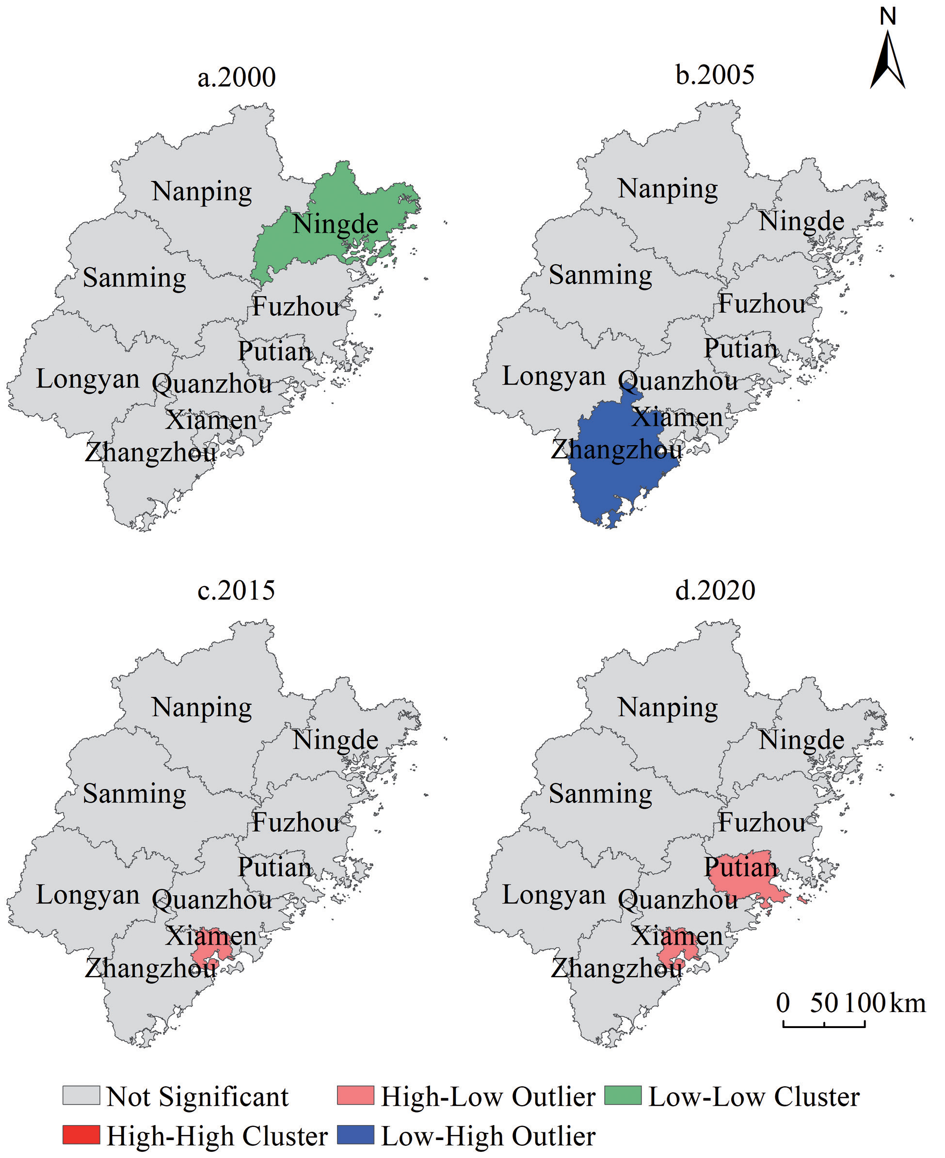
Table 6.
Parameters associated with the GTWR model regression.
| Model Parameters | Bandwidth | Residual Squares | Sigma | AICc | R2 | R2 Adjusted | Spatio-temporal Distance Ratio |
|---|---|---|---|---|---|---|---|
| value | 0.116 | 10.129 | 0.232 | 147.187 | 0.946 | 0.945 | 0.269 |
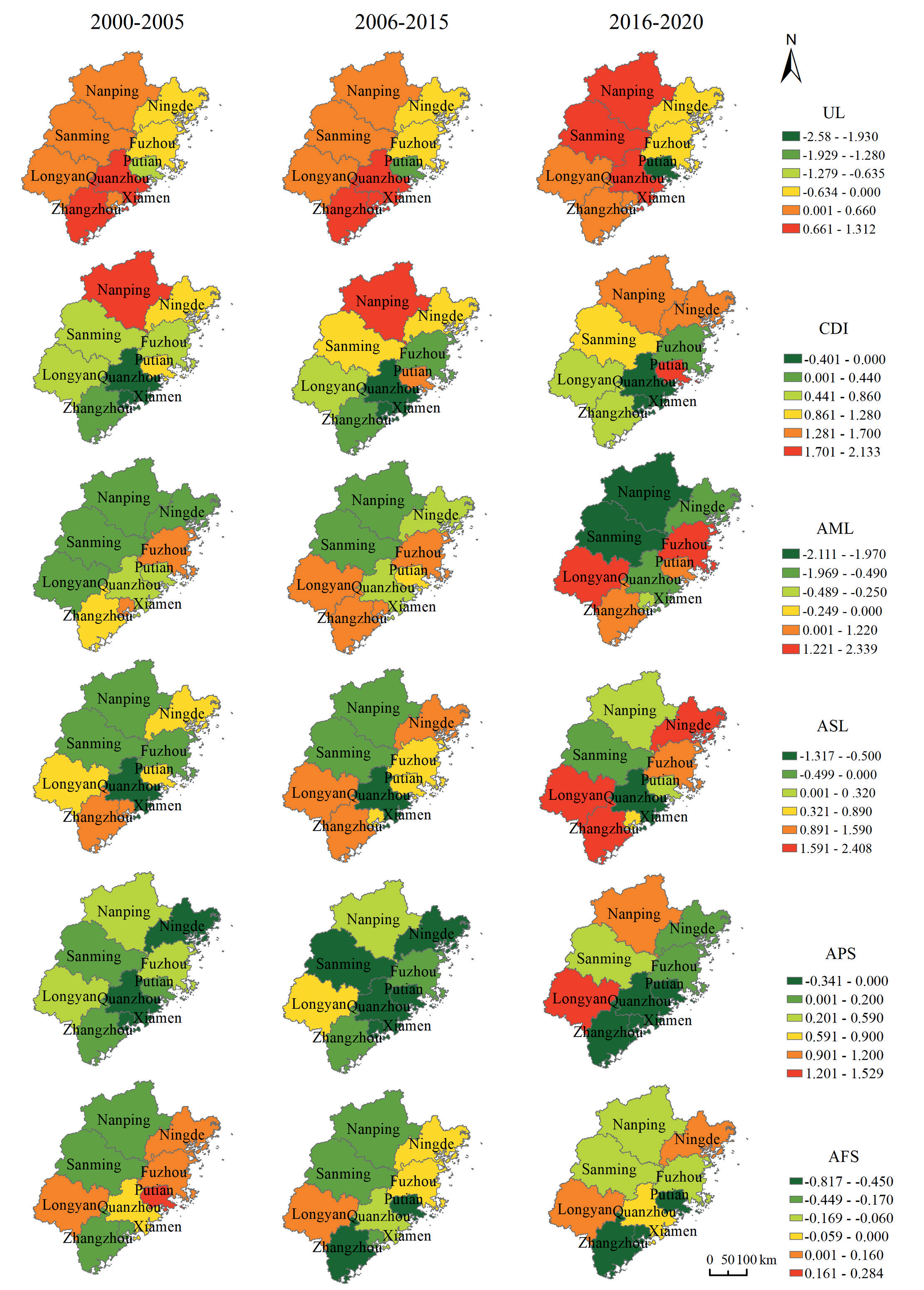
There are spatial differences in the inflluence of various factors on AEE in Fujian Province in different periods, as follows:
(1) The regression coefficients of the urbanization rate mainly show an increasing pattern from the northeast to the southwest, and the urbanization rate has the greatest positive impact on the AEE of Quanzhou, Xiamen, Sanming, and Nanping, while it has a negative impact on Putian, Fuzhou, and Ningde. On the one hand, the increase urbanization rate promotes the consumption upgrading of urban residents and increases the demand for green agricultural products, and farmers pay attention to the protection of agricultural ecology and reduce the use of pesticides and chemical fertilizers. On the other hand, it brings advanced environmental concepts to influence farmers’ production behavior choices and improve AEE. However, at the same time, increasing urbanization has led to an expansion of consumer demand for all kinds of resources and an increase in agricultural carbon emissions, which has also led to an exodus of high-quality labor from the countryside, and the ageing and low quality of the agricultural labor force may have led farmers to adopt non-green production methods, thereby reducing AEE, similar to what Zhao et al. argued [38].
(2) The regression coefficients of farmers' income levels show a pattern of increasing from southeast to northwest. The regression coefficients remain positive for all cities except Xiamen and Quanzhou. The effect of farmers’ income level on AEE then increases over time in Putian, Zhangzhou and Ningde cities. The main reason for this is that as farmers’ incomes have increased, they have begun to shift to organic and sophisticated agriculture, are more receptive to advanced agricultural concepts and production techniques, and are more capable of changing their old sloppy production behavior, thus improving AEE.
(3) The regression coefficients of mechanization mainly show a decreasing trend from central and southeastern Fujian to the periphery. The positive effect of mechanization on AEE is increasing in Longyan, Fuzhou, Putian and Zhangzhou.The regression coefficients of Longyan, Putian and Zhangzhou change from negative to positive. In Xiamen, the regression coefficients turn from positive to negative, and the negative impact of mechanization level on AEE is reinforced in Sanming, Nanping and Quanzhou, possibly because the increase in the level of agricultural mechanization is often accompanied by a large consumption of resources, which increases undesired outputs and thus reduces AEE. The result suggests that the level of agricultural mechanization has a two-way effect on AEE [47].
(4) The regression coefficients of agricultural resource endowment show an increasing pattern from the center to the southwest and northeast. The positive contribution of agricultural resource endowment to AEE is greater in Longyan, Zhangzhou and Ningde, followed by Fuzhou and Xiamen, and finally Putian. The likely reason for this is that the larger the area sown to crops per capita, the easier it will be to achieve an appropriate scale of operation, thereby increasing the utilization rate of the means of agricultural production and contributing to the improvement of AEE [48]. The regression coefficients of Quanzhou, Sanming and Nanping are negative, which may be attributed to the fact that the larger the area sown to crops per capita, the more unfavorable it is for the fine management of crops, leading to the waste of resources and a reduction in eco-efficiency. This may be indicated by the results of Grzelak [37].
(5) The regression coefficients for agricultural cropping structure increase from the east to the west. The positive effect of agricultural cropping structure on AEE in mountainous areas increases with time. This result is consistent with the findings of Zeng et al. [49]. The high proportion of sown area of grain crops in the mountainous areas of western Fujian Province is likely to bring about a scale effect, which is conducive to the specialized division of labor, and to the accumulation of experience and upgrading of skills by farmers, thus improving AEE.
(6) The regression coefficients for the level of financial support for agriculture show a pattern of higher in the northeast and southwest and lower in the middle. The level of financial support for agriculture has the largest negative impact on Zhangzhou, followed by Nanping and Sanming, and gradually weakens, the coefficient of Ningde shows a trend of decreasing and then increasing, and the regression coefficients of Putian and Fuzhou experience a shift from positive to negative. The reason for this is that reasonable financial expenditure on agriculture can lead to scientific and technological innovation, enhance the training of talents, promote the transformation of agricultural production methods, and help improve regional AEE [10]. However, when the government’s financial support for agriculture involves the ecological environment, due to the public good nature of the ecological environment, externalities tend to occur, resulting in market failures and the inability to allocate resources reasonably, leading to a decline in AEE [50].
Conclusion and Discussion
(1) AEE in Fujian Province is generally increasing, albeit with notable inter-regional disparities. This trend may be attributed to the ongoing exploration of modern agricultural development paths and the successful implementation of green agricultural practices. This coincides with the research results of our team [51]. However, the AEE varied greatly among different regions. This is strongly related to the redundancy of inputs in some regions, resulting in excessive agricultural carbon emissions. It is recommended to actively explore the effective combination with the "carbon trading market", establish a market-based and diversified agro-ecological compensation mechanism, and guide farmers to adopt green production methods in agriculture to achieve low carbon emissions in agriculture and improve AEE.
(2) Spatially, the AEE in Fujian Province exhibits a stochastic spatial distribution pattern, albeit with localized clustering. It is worth noting that there was no occurrence of the H-H aggregation phenomenon of AEE in Fujian Province from 2000 to 2020. This indicates that a large-scale aggregation of high values has not yet formed in the province and that Xiamen, which has a higher AEE value, does not significantly impact the AEE of neighbouring cities. Therefore, interregional coordinated development still requires strengthening. It is imperative that Fujian Province actively pursues the inter-regional synergistic green development model to promote sustainable and coordinated agricultural development across the region.
(3) Overall, the AEE of Fujian Province is positively influenced by the factors of farmers’ income and agricultural resource endowment, while negatively impacted by the level of agricultural mechanization. The inhibitory effect of urbanization development on AEE is increasing progressively. However, there is also a positive effect on the mountainous areas of Fujian and southern Fujian, which verifies the intricate influence of urbanization on AEE [52]. Contrary to common belief, elevating the levels of financial aid for agriculture could impede AEE. Additionally, the manner in which different factors promote AEE displays noteworthy spatial disparity. Urbanization possesses the most detrimental effect on Putian, while the level of agricultural mechanization impacts Fuzhou, Sanming, and Nanping, but in different directions. Agricultural resource endowment has a positive impact on Zhangzhou, Longyan, and Xiamen, but has a negative impact on Quanzhou. Meanwhile, farmers’ income primarily influences Ningde positively. Therefore, it is crucial for Fujian Province to establish a tailored agroecological developmental plan that aims to improve the efficiency of agricultural practices in each area.
There are also some shortcomings in the article. Specifically, it should fully take into account that agricultural development is a complex system involving nature, society, economy and culture, and include more elementary variables such as relevant policies and changes in agricultural technology in order to scientifically analyze the main drivers of AEE. In addition, the specific mechanism of each driver needs to be further explored in depth, which is also a direction where future research can go deeper.

