

Introduction
In recent decades, human activities (such as deforestation) and global climate anomalies (such as global warming) have increased both the frequency and severity of forest disturbances. Accurately and consistently grasping information on forest disturbances is crucial for forest management, climate change analysis, and carbon accounting [1-4]. Large-scale satellite images provide ideal observations for the dynamic monitoring of forest disturbances on both regional and global scales [5, 6]. Mapping forest disturbances using remote sensing time series has gained significant attention [7-11], as this dynamic analysis improves both operational efficiency and mapping accuracy by leveraging temporal context.
Different types of forest disturbances cause varying magnitudes of change in spectral bands or indices. For example, the change magnitude of the forest spectrum resulting from clearcut is obviously higher than those resulting from insects and degradation [12, 13]; change magnitudes in the Normalized Burn Ratio (NBR) caused by logging and fire are similar, but both are greater than those resulting from road construction and insects [14]; harvest tends to display Shortwave infrared 1 (SWIR1) band values that are higher than that following fire [15]. Disturbance detection accuracy is closely related to the disturbance type and change magnitudes in spectral band or index. High-magnitude disturbances, like harvesting and fire, are easier to detect [16]. However, most general change detection algorithms, such as Breaks For Additive Seasonal and Trend (BFAST), Continuous Change Detection and Classification (CCDC), and LandTrendr, are designed for stand-replacing disturbances with high magnitudes [17- 20]. Consequently, these algorithms may not effectively detect low-magnitude disturbances (such as early-stage insect infestations, diseases, and selective logging) that do not significantly alter forest composition, structure, or condition. For example, Rodman et al. [16] found that wildfire is detected more accurately than insect-induced tree mortality using the LandTrendr algorithm. The main reasons for the low detection accuracy for low-magnitude forest disturbance agents are as follows: the spectral responses to low-severity disturbances are subtle [21]; gradual and low-severity disturbances may be confounded and even covered by forest phenology and atmospheric effect [16, 22]. Detecting low-magnitude disturbances is crucial, as it forms the foundation for simultaneously detecting various disturbance agents with different change magnitudes. Therefore, detecting subtle changes in forest ecosystems using remote sensing time series has become a growing interest [23], and several algorithms aimed at detecting low-magnitude disturbances have been proposed [24-27]. For example, Meng et al. [25] discriminated between insect-induced tree mortality and undisturbed forest using the threshold-based method and further detected low-moderate severity areas using spectral-temporal anomaly information. Ye et al. [27] developed a CCDC-like algorithm to detect forest insect disturbances. However, most of these algorithms, which are designed for specific low-magnitude disturbance types, require setting a fixed threshold for change magnitude. Additionally, optimizing this threshold requires adequate disturbance samples, which can be difficult and time-consuming to collect. Furthermore, the effectiveness of detecting high-magnitude disturbances using these algorithms designed for a specific low-magnitude disturbance type remains uncertain. When multi-type forest disturbance agents with different change magnitudes occur in a large-scale forest over a long period, existing change detection algorithms designed to detect a specific low- or high-magnitude forest disturbance may not fully capture all scenarios[28].
COntinuous monitoring of Land Disturbance (COLD), the first disturbance mapping algorithm, was designed to detect multi-type disturbances. It significantly improves the detection of subtle changes while still effectively detecting drastic changes [29]. However, the omission errors for low-magnitude disturbance agents are still relatively high (~40%). As one of the key tools in the field of statistical process control, the Exponentially Weighted Moving Average (EWMA) chart is sensitive to small shifts when the smoothing parameter λ in the chart that determines the threshold for change magnitude is set as small. Brooks et al. [30, 31] proposed the EWMA Change Detection (EWMACD) algorithm to identify both clearcut and selective logging using remote sensing time series, successfully detecting diverse disturbance agents with different change magnitudes simultaneously. Although the EWMA chart with a small size of λ allows for detecting both low- and high-magnitude disturbances, it will cause a potential temporal delay in detecting sudden high-magnitude disturbances. This is because assigning less weight (small λ value) to the current disturbance signal with a high negative value prevents the EWMA chart value from exceeding the control limits promptly, a phenomenon known as the “inertia problem” [32]. This means a single EWMA chart with a fixed λ cannot effectively detect both low- and high-magnitude disturbances simultaneously. The adaptive detection method has significant advantages as it can dynamically adjust parameters based on data changes, thereby more accurately reflecting the current state [33-35]. In order to overcome the inertia problem of traditional EWMA charts, an adaptive EWMA (AEWMA) chart has been developed, which can respond more flexibly to the interference of different amplitudes and provide timely detection results. The AEWMA chart adaptively optimizes the smoothing parameter λ according to the shift size [32]. When the shift size is large, the smoothing parameter λ adapts by increasing in size. More weight is then assigned to the current disturbance signal with a high negative value. As a result, the sudden drop in the current AEWMA chart value allows for quickly detecting high-magnitude disturbances. Because the AEWMA chart is superior to the ordinary EWMA chart in detecting different shifts when the shift size is unpredictable [36], it has the potential to accurately detect low- and high-magnitude forest disturbances using remote sensing time series. Research has confirmed the potential of using the AEWMACD algorithm to detect various forest disturbances [37].
Change detection algorithms using dense time series generally eliminate the interference of phenological variations in detecting disturbance using the harmonic model to describe the seasonal changes. However, Landsat time series in cloudy and rainy subtropical or tropical regions are acquired with a low temporal frequency (sparse) of clear observations at an irregular interval [38], which may cause over-fitting of the harmonic model during the training stage [39]. Meanwhile, online change detection algorithms (such as BFAST, CCDC, COLD, and EWMACD) establish control limits or a boundary of the observations’ empirical fluctuation (i.e. threshold) depending on an accurate estimation of the standard deviation of fitting residuals during the training stage. However, the standard deviation estimator based on sparse observations may also be inaccurate, leading to a deterioration in the performance of the change detection algorithms. Thus, those algorithms using dense time series are inapplicable in frequent cloud cover regions. To overcome these problems, Wu et al. [40] adopted spatial normalization to remove forest phenological variations, reducing the need for dense observations during model initialization. Then, EWMA-t [41], a combination of EWMA and t charts for short cycles (sparse observations), was introduced to propose the EWMA-t change detection (EWMATCD) algorithm. This algorithm quickly establishes reliable control limits based on limited images for forest disturbance detection. Compared to the EWMACD algorithm, the EWMATCD algorithm enables the detection of both low-intensity and high-intensity disturbances, even in cloudy and rainy subtropical regions based on sparse observational data. However, similar to the EWMA chart, the inertia problem can also result in a temporal delay in detecting high-magnitude disturbances by using the EWMA-t chart with a fixed small value of λ. More seriously, the inertia problem may even result in a higher omission error rate for the high-magnitude disturbances in regions with insufficient data if the disturbance agent is only visible for a few observations because of the requested amount of consecutive out-of-control signals for determining disturbance.
In this article, we aim to detect various forest disturbance types with different change magnitudes in regions with low data availability. This article’s diverse disturbance agents include both high-magnitude disturbances (clearcut and fire) and low-magnitude disturbances (selective logging and insects). To achiteve the objective, AEWMA-t change detection (AEWMATCD) algorithm based on the AEWMA-t chart proposed by Chang and Sun [42] was first developed to accurately detect the target disturbance agents through adaptively optimizing smoothing parameters for different disturbance agents using sparse Landsat time series. Then, with a comparison to the EWMATCD algorithm with an inertia problem, the ability of AEWMATCD to detect diverse disturbance agents was evaluated, and the differences in detection accuracy among diverse disturbance agents were analyzed.
Materials and Methods
Study Area
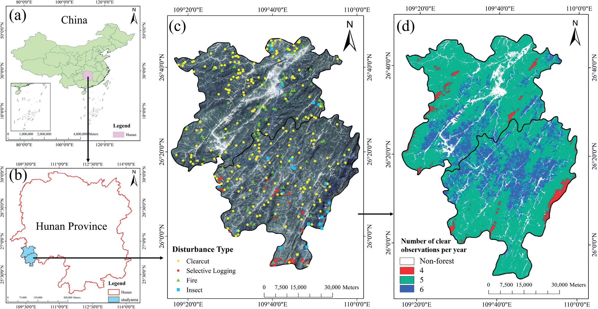
The study area, comprising the counties of Jingzhou and Tongdao, is located southwest of Hunan Province, China (Fig. 1(a-c)). These counties are key forested regions of China, with forest coverage rates exceeding 70%. The subtropical monsoon humid climate in the study area leads to frequent cloudy and rainy weather, contaminating satellite optical data and forming sparse Landsat time series. Due to severe karst rocky desertification, the forest ecosystem in the study area is fragile and highly susceptible to climate change and human activities. The primary forest disturbance targets for detection in this study area include deforestation (such as clearcut and selective logging), insects, and fire, which lead to different change magnitudes in the forest spectrum. Hence, this study area provides an ideal condition for verifying the feasibility of detecting diverse disturbance agents from sparse Landsat time series using the proposed AEWMATCD algorithm.
Landsat Data and Forest Benchmark Mask
Landsat TM5, ETM+7, and OLI8 surface reflectance (SR) time series from 2001 to 2020, consisting of 115 images with less than 20% contaminated pixels, was collected from the US Geological Service (USGS). The three datasets are coordinated in a sequential order based on time. The annual average number of clear observations for 78.5% of pixels is 5 (Fig. 1d)), which is insufficient to construct a reliable harmonic model to eliminate the interference of phenological changes. The SLC-off gaps in the ETM+7 images were filled using a spatiotemporal interpolation method [43], and the function of mask products (Fmask) was applied to mask out clouds and cloud shadows. A forest benchmark mask was delineated using the random forest classification algorithm based on the Landsat image taken on October 3, 2002 (the date corresponding to the maximum training length for most forest pixels), to remove the non-forest pixels (Fig. 1d)). The forest benchmark mask maximizes the likelihood of selecting forest pixels as analysis targets and minimizes the possibility of stand-replacing disturbances occurring during the training stage.
Validation Data
The validation dataset, consisting of 345 disturbed plots (Fig. 1c)) and 345 undisturbed plots, were collected to evaluate the detection accuracy of the AEWMATCD algorithm. The type and initial disturbance date for each disturbed plot in the Landsat time series were determined through visual interpretation of the time series data (multispectral composite images and time series curves) and high-resolution images acquired from Google Earth, supported by additional materials. Specifically, MODIS MCD14ML active fire product was used to assist in collecting fire samples; insect samples were collected assisted by local historical statistics and relevant news and articles; and the clearcut and selective logging samples entirely collected relied on visual interpretation of Landsat time series data and high-resolution images. Finally, a total of 345 disturbed plots, including 219 clearcut, 40 selective logging, 59 fire, and 27 insect samples separately, were collected. In addition, 345 undisturbed plots were sampled from the non-disturbance forest region, which were also confirmed using Landsat time series data and Google Earth imagery.
Methodology
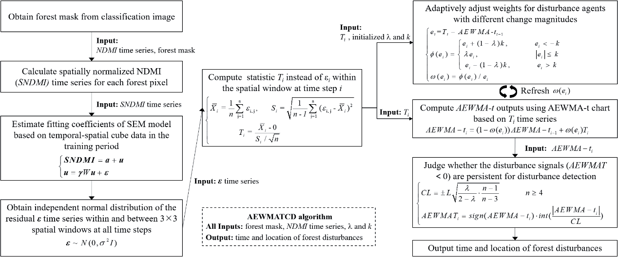
The flowchart of detecting diverse forest disturbance agents with different change magnitudes using the proposed AEWMATCD algorithm is shown in Fig. 2. First, to eliminate the interference of forest seasonal variations in disturbance detection, the Normalized Difference Moisture Index (NDMI) was spatially normalized using the spatial context to finish subsequent model initialization using sparse clear observations. Second, in order to meet the requirement for AEWMA-t chart input to follow an independently normal distribution in both the temporal and spatial dimensions, the spatial errors model (SEM) was established through fitting temporal-spatial observations in the training stage. The residual time series were then generated by subtracting the observed values from the fitted values, yielding normally distributed residuals. Third, the residual time series were input to the AEWMA-t chart to detect diverse disturbance agents, and disturbances were labeled if the AEWMA-t values consecutively exceeded the control limits. The crucial procedures are described in more detail in the following sections.
Spatial Normalization of NDMI for Model Initialization
By contrasting SWIR1 and NIR bands, NDMI (1) [44] has been proven to be sensitive to forest insects [25, 27, 45]. NDMI has also been widely used in detecting deforestation, including clearcut, small-scale deforestation, and selective logging [7, 9, 10, 46, 47]. In addition, NDMI also has the ability to detect fire [48- 50]. Therefore, NDMI was selected as the spectral input of the change detection algorithm for detecting diverse forest disturbances with different change magnitudes, including clearcut, fire, selective logging, and insects in this study.
NDMI was calculated as:
To reduce the impact of phenological variations on change detection, the spatially normalized NDMI (SNDMI) was calculated as (2). First, NDMImedian was then obtained by calculating the median NDMI of the pixels exceeding a certain percentile P (set to 90% in this study) within a moving window. Then, the SNDMI of the central pixel was obtained by dividing the NDMI value of the central pixel (NDMIpixel) by NDMImedian. This approach assumes that the upper tail of the pixels within the moving window are forested, and their seasonal variations are similar to that of the central pixel. Therefore, SNDMI can remove the phenological variations. SNDMI time series were calculated from 2001 to 2020 for each forest pixel.
The spatial moving window size is important for normalization. Based on the analysis of the collected sample data and statistical data on insects and fires in the study area, the areas of forest deforestation, fire, and insect patches are generally smaller than 35 ha. Therefore, the window size was set to 21Í21 pixels (39.69 ha) to avoid smoothing out the impact of disturbances when calculating the spatially normalized index while preserving the temporal dynamics similarity between the central and neighboring pixels.
Considering that the SNDMI time series has eliminated the seasonal changes described by a harmonic model in previous studies, the harmonic model was superseded by a simple linear model (3).
where a is theoretically close to 1 and estimated using ordinary least squares, and ui is the residual at date ti. Fitting the simple linear model requires only six clear observations [51], thereby shortening the length of the training stage in regions with insufficient data.
Acquisition of Independently Normally Distributed Residual Time Series Using SEM Model
Diverse forest disturbance agents were detected using the AEWMA-t chart, which requires the input data in the temporal-spatial domain to follow an independently normal distribution. However, due to strong spatial correlation, the assumption that the n spatially adjacent residuals at the same time step follow an independently normal distribution may fails [52]. Therefore, instead of (3), SEM (4) was performed to remove the spatial correlation of the regression residuals:
where SNDMI denotes SNDMI observations with the size of m (length of time series) Í n; a represents n regression coefficients a; u represents the matrix of spatially correlated regression residuals ui; γ is the spatial dependence parameter estimated by maximum likelihood method; W is the spatial weight matrix filled with 1 for neighboring forest pixels and 0 otherwise; ε is the independently normally distributed residuals in the temporal-spatial domain, and I denotes the identity matrix. Therefore, instead of the regression residuals ui estimated by the simple linear model (3), the independently normally distributed residuals ε can be entered into the AEWMA-t chart for disturbances detection.
The training stage is limited to six time steps, which reduces the likelihood of disturbances occurring and affects fitting accuracy. To avoid a disturbance or noise during the training stage, we adopted the approach of [20, 31]: a moving window with six time steps, initially sequentially until the fitting accuracy reached the required precision R2min (0.7) or the window moves to the date corresponding to the maximum training length (12 time steps). Since some outliers or contaminated pixels in the training stage may be not removed by using Fmask, a two-step fitting procedure was employed for each model fitting: 1) all clear observations within the moving window were utilized to fit the SEM model, 2) the SEM model was fitted again by using the remaining observations after removing the observations whose fitting residuals ε are greater than three times the standard deviation of all residuals at the first time.
Diverse Disturbance Agents Detection Using AEWMA-t Chart
EWMA-t chart, designed for short production runs, can detect outliers using limited samples. Some studies have proven that the EWMA-t chart has the ability to detect forest disturbances in cloudy and rainy regions [40]. To build the reliable control limits using a limited number of observations, the statistic Ti replaced the residual εi in [30] and is treated as the input for the EWMA-t chart:
where Xi represents the subgroup mean, and Si represents the standard deviation of subgroups εi,n at date ti. Therefore, the EWMA-t statistic, EWMA-ti is defined as:
where the smoothing parameter λ, ranging from 0 to 1, is used to measure the retrospective nature of the chart. Specifically, more weight is assigned to the current residual statistic (Ti) when λ is close to 1, and the EWMA-ti value principally depends on previous values EWMA-ti-1 when λ is close to 0. The initial value of EWMA-t0 is normally set to 0.
Based on the principle of effectively detecting low-magnitude disturbances, the value of λ was set to a small value of 0.25, which is one of the determining factors of the control limits (CL) (7). The forest pixels within the 3Í3 patch were labeled as disturbed if EWMA-ti crosses the lower CL [53]. The value of L was set to 2.
The EWMAT index was calculated to signal disturbances (8).
where sign() is a sign function , || represents the absolute value, and int[] is used to round down the absolute value. A forest patch is marked as undisturbed if its EWMAT value is equal to 0, and a possible disturbance occurs when the EWMAT value is less than 0.
Similar to the EWMA chart, the inertia problem of the EWMA-t chart with a fixed small value of λ (0.25) will also cause a temporal delay in detecting high-magnitude disturbances. For resolving the ‘inertia problem’, the AEWMA chart where smoothing parameter λ is adaptively optimized according to the change magnitude has been developed [32], and this adaptive strategy is also introduced to the EWMA-t chart to establish the AEWMA-t chart (9) [42].
where ei =Ti -AEWMA-ti-1 is the estimation error. ϕ is the function of ei, and a widely used score function (10) was adopted [32].
where k is the deviation threshold and was set to 3 in this study. Using the definition of ω(ei) = ϕ (ei)/ei, AEWMA-t chart can be rewritten as follows:
ω(ei) is equivalent to the smoothing coefficient λ in (6). ω(ei) is equal to λ and the AEWMA-t chart was converted to EWMA-t chart when there is a low-magnitude disturbance in the process (|ei|≤k). When a low-magnitude disturbance occurs (|ei|≤k), the score function makes the equivalent smoothing coefficient ω(ei) smaller. Because the lower CL’s absolute value is small, AEWMA-ti can exceed the lower CL, which means the AEWMATCD algorithm is sensitive to low-magnitude disturbances. Conversely, when a high-magnitude disturbance agent occurs (ei<-k), the sudden drop in the current chart value AEWMA-ti makes the high-magnitude disturbance quickly detected, effectively overcoming the inertia problem and making the algorithm suitable for detecting both low- and high-magnitude disturbances. The AEWMAT index was calculated to signal disturbances:
Like the EWMA-t chart, a forest patch is labeled as undisturbed if its AEWMAT value is equal to 0, and a possible disturbance occurs if the AEWMAT value is less than 0. A disturbance is determined when consecutive out-of-control signals are detected, effectively lowering the false positives due to ephemeral factors, such as clouds that were not removed by Fmask [20, 30]. The number of consecutive out-of-control signals for determining disturbance is half of the annual average number of clear observations [31]. Considering the small size of the forest patch, the likelihood for the rest within the patch to be disturbed subsequently is high when some forest pixels are disturbed at the current time step. Therefore, the current time step is treated as the occurrence time of forest disturbance in the patch.
Results
Feasibility Analysis of Detecting Diverse Disturbances in Sparse Landsat Time Series Using AEWMATCD Algorithm
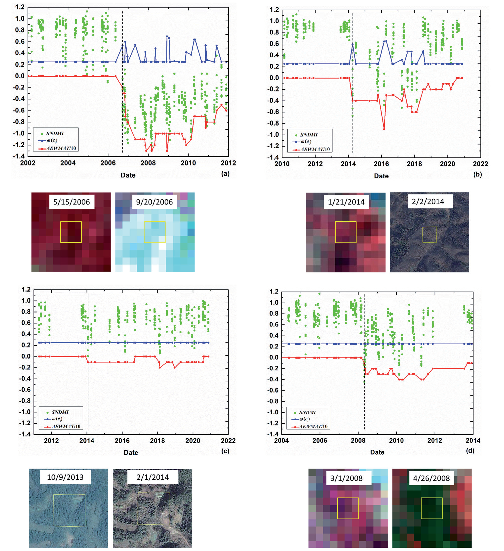
AEWMATCD algorithm was performed to detect clearcut, fire, selective logging, and insect agents separately to analyze the feasibility of detecting diverse disturbances (Fig. 3). Because clearcut and fire agents both result in stand-replacing transition, change magnitudes of SNDMI for clearcut (the SNDMI median of the pixels within the patch dropped from 0.80 to -0.54) and fire agents (dropped from 0.83 to -0.19) were both high (Fig. 3(a-b)). When clearcut or fire agent with high-magnitude occurred, the equivalent smoothing coefficient ω(ei) adaptively get larger from initial 0.25 to 0.53 for clearcut and from initial 0.25 to 0.59 for fire. Then a sudden drop in the current chart value AEWMA-ti with more weights makes current AEWMAT value quickly less than 0 (-2 for clearcut and -4 for fire). The high-magnitude disturbances quickly detected, effectively overcoming the inertia problem. Selective logging or insect agents leads to subtle changes in structure or condition with a persisting forest cover and, therefore, change magnitudes of SNDMI for selective logging (the SNDMI median of the pixels within the patch dropped from 0.72 to 0.35) and insect agents (dropped from 0.76 to 0.12) were both low (Fig. 3(c-d)). When selective logging or insect agents with low magnitude occurred, ω(ei) still kept a small value (initial λ=0.25). Because the absolute value of the lower CL is small, it makes the current chart value AEWMA-ti can cross the lower control limits, and the current AEWMAT value less than 0 (-1 for both selective logging and insects), which means the AEWMATCD algorithm is sensitive to selective logging or insects agent with low-magnitude. The results proved that the AEWMATCD algorithm is feasible for detecting both low- and high-magnitude disturbances based on the adaptive adjustment of the smoothing coefficient ω(ei) for different change magnitudes.
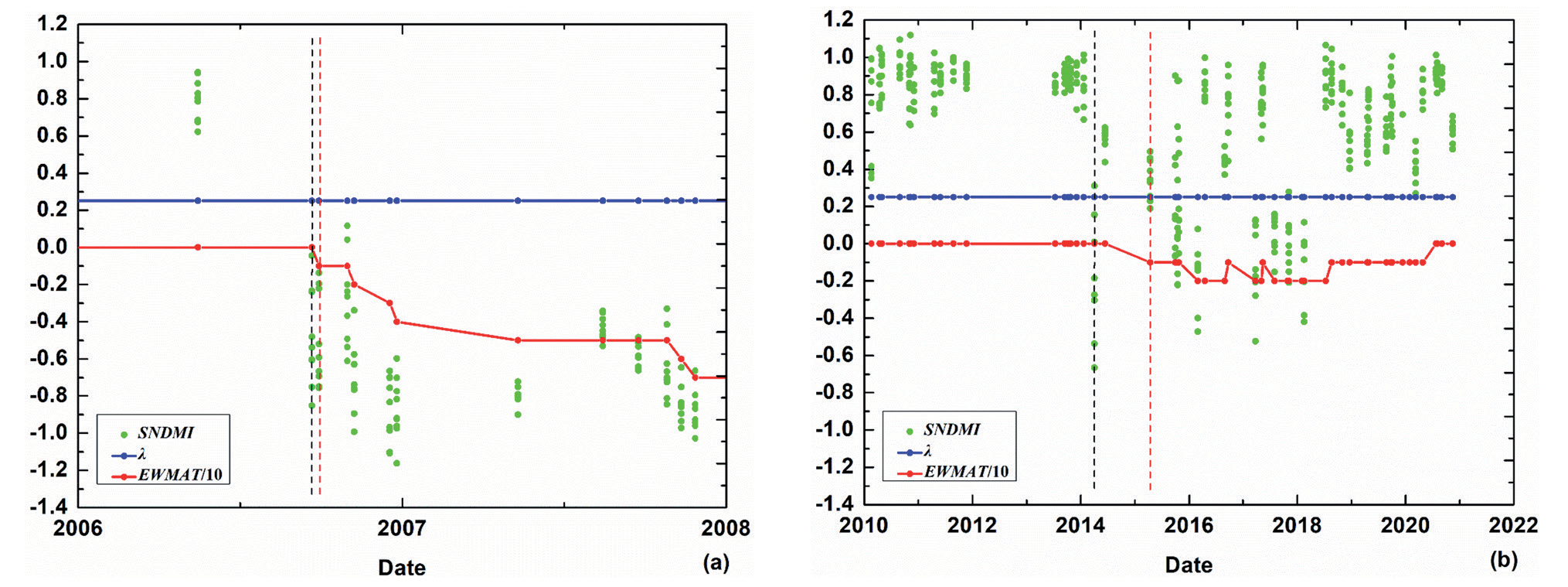
To verify the applicability of the AEWMATCD algorithm to detect disturbances using sparse Landsat time series, the AEWMA chart was performed to detect the clearcut agents in Fig. 3a), wherein the annual average of clear observations is equal to 5, for comparing with the result using the AEWMATCD algorithm (Fig. 4). Like the EWMA chart in Brookes et al. (2014), the AEWMA chart also needs dense, clear observations to establish a reliable baseline by fitting the harmonic model during the training stage and control limits that depend on an accurate estimation of the standard deviation of fitting residuals. However, when the observations at six time steps, the same number of time steps used to estimate 1 fitting parameter in (4) in the AEWMATCD algorithm were applied to fit the harmonic model with 2 harmonic terms (i.e. 5 fitting parameters) in AEWMA chart, overfitting of the harmonic model influenced the removal of seasonality. This resulted in an inaccurate estimation of the standard deviation of fitting residuals, which led to false alarms (or omission errors) (Fig. 4a)). Although the AEWMA chart can accurately detect disturbances when the observations at 15 time steps that are thrice larger than 5 fitting parameters were used (Fig. 4b)), the long training stage with nearly 4 years in this sample introduces the challenge in online detecting multiple disturbances in regions with low data availability or with frequent disturbances. On the contrary, the proposed AEWMATCD algorithm only needs the observations with the size of 3Í3 (spatial window) Í6 (time steps) to fit the SEM model. Then, it can accurately detect the clearcut agent (Fig. 3a)). Therefore, the AEWMATCD algorithm can also detect disturbances in regions with insufficient data.
To further assess the ability to overcome the delay in detecting high-magnitude disturbances using the proposed AEWMATCD algorithm, the EWMATCD algorithm and the EWMA-t chart with a fixed small value of λ (0.25) were executed on the high-magnitude disturbance agents in Fig. 3(a-b) (Fig. 5). Compared with the result of timely detection using the AEWMATCD algorithm, the disturbance was detected with the delay of one or two time steps when the EWMATCD algorithm was executed. More seriously, when the disturbance agent was only recorded on the limited time steps of the time series because of low data availability, the limited clear observations and inertia problem of the EWMA-t chart led to the number of consecutive signals crossing the CL for labeling disturbances not enough, resulting in omission error. As shown in Fig. 6, clear observations at only three time steps (corresponding to the second, third, and fourth dashed lines) were recorded in the duration of a clearcut agent, and the inertia problem of the EWMA-t chart resulted in the lack of three consecutive out-of-control signals for determining disturbance (Fig. 6b)). Meanwhile, the AEWMATCD algorithm can detect the clearcut agent in a timely manner, even if clear observations are limited (Fig. 6a)).
Assessment of Disturbance Detection Accuracy in the Spatial Domain
The assessment results of the spatial accuracy of detecting disturbances using the AEWMATCD algorithm was shown in Table 1. The producer’s and user’s accuracies for the undisturbed samples are 80.0% and 88.2%, respectively, while those for the disturbed samples are 89.3% and 81.7%, respectively. The absolute value of the lower CL is set as a low value for effectively detecting the low-magnitude disturbances, and therefore, the commission error rate (69/377 = 18.3%) is larger than the omission error rate (37/345 = 10.7%) for the disturbances. The overall accuracy of 84.6% indicates that the AEWMATCD algorithm can effectively detect diverse disturbance agents with different change magnitudes.
Fig. 3.
Detection of diverse forest disturbance agents within the 3×3 spatial window (yellow boxes in high-resolution images or Landsat images before and after disturbance) using the proposed AEWMATCD algorithm: a) clearcut, b) fire, c) selective logging, and d) insects. The dashed lines in the AEWMA-t chart represent the initial dates of disturbances labeled by AEWMATCD algorithm. RGB: R= band NIR, G=band Red, B=Green. We displayed Google Earth Pro (GEP) images if the date near the disturbance occurs has available images for better intuitiveness.
Considering each disturbance type (Table 1), the producer’s accuracy is highest for clearcut (92.7%), and it was followed by fire (89.8%), which means that a high proportion of high-magnitude disturbance agents were correctly detected (low omission error). Although the producer’s accuracy was relatively low for selective logging (80.0%) and insects (74.1%) compared to clearcut and fire, disturbance detection was still moderately successful for low-magnitude disturbance agents. A comparison of different disturbance agents showed expected patterns of detection accuracies for high-magnitude disturbances that were higher than low-magnitude disturbances.
Fig. 4.
Detection of forest clearcut agent in Fig. 3a) using AEWMA chart: the number of training data is equal to a) 6 and b) 15, respectively. The dashed line in the picture represents the clearcut date labeled by the AEWMA chart.
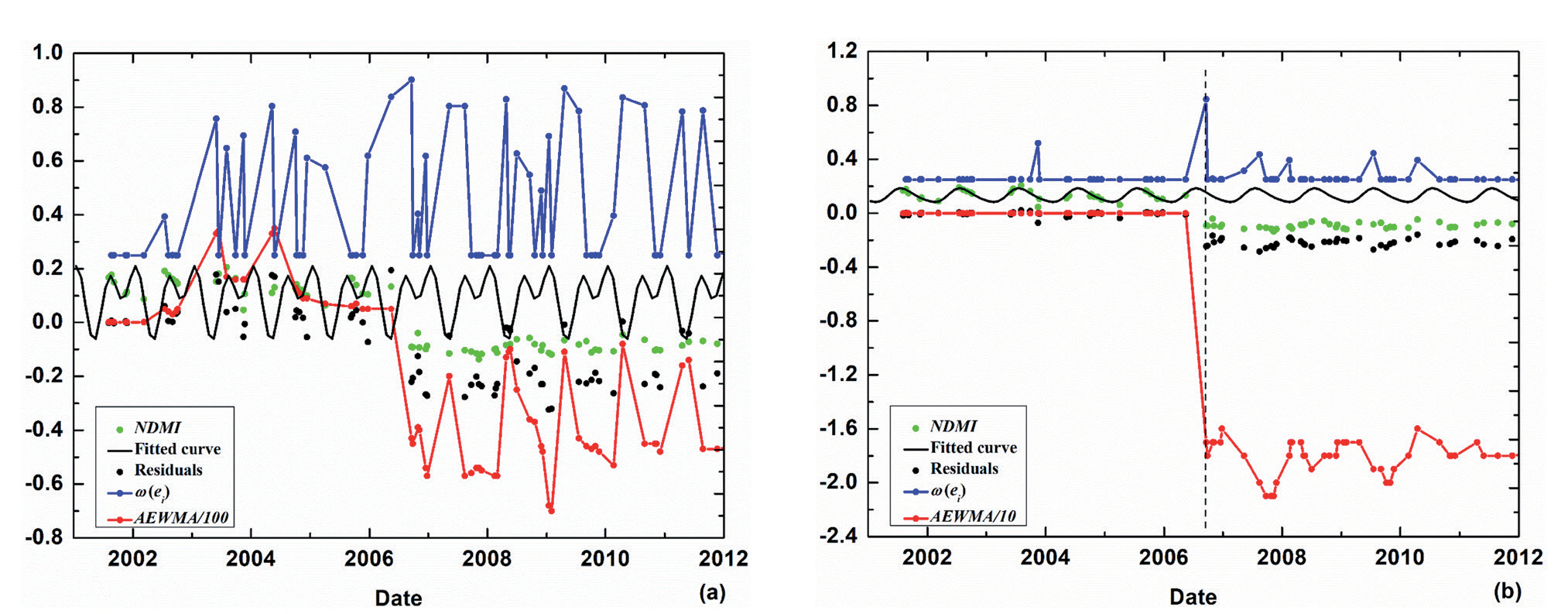
Fig. 5.
Detection of forest high-magnitude disturbance agents in Fig. 3(a-b) using EWMATCD algorithm: a) clearcut, b) fire. The black and red dashed lines in EWMA-t chart represent the initial dates of disturbances and the dates of disturbances detected by the EWMATCD algorithm, respectively.
Most of the commission errors can be ascribed to:
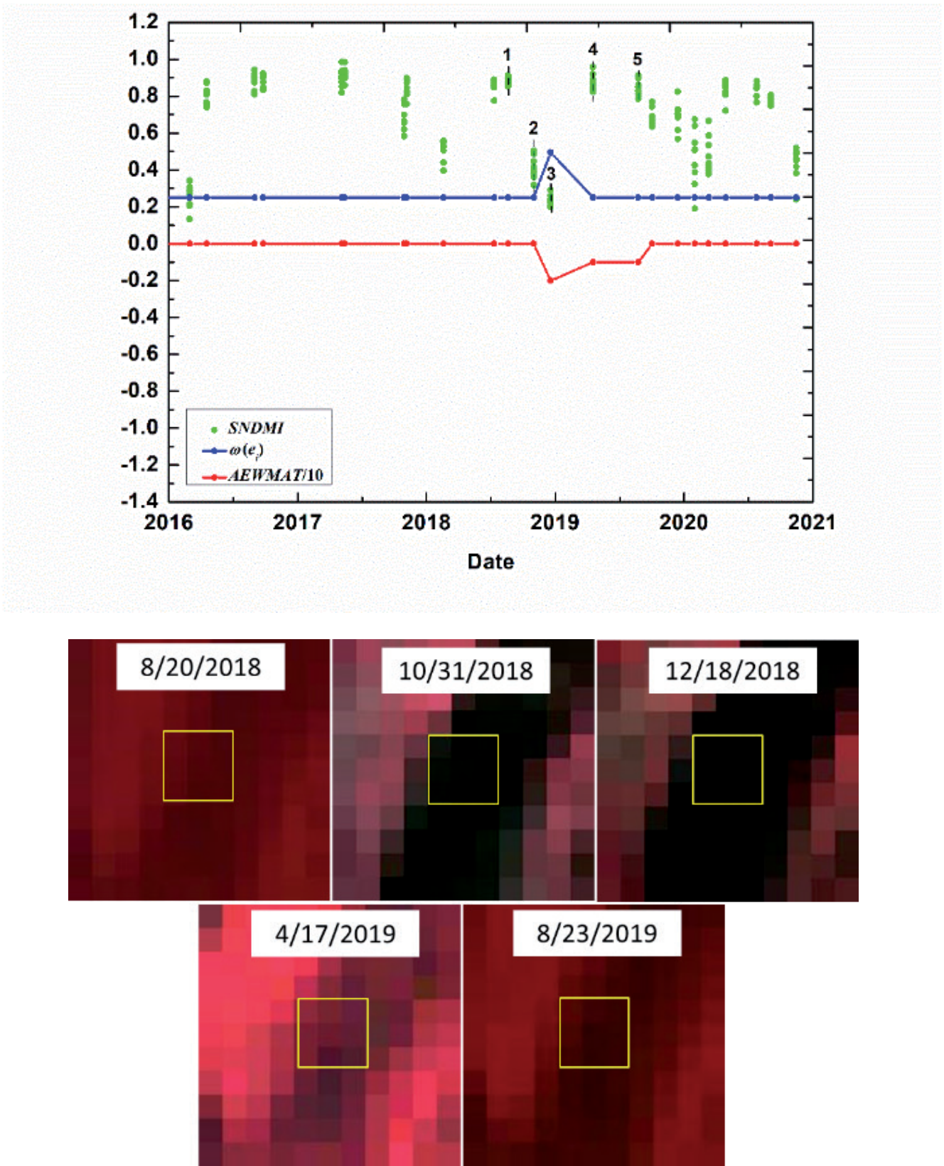
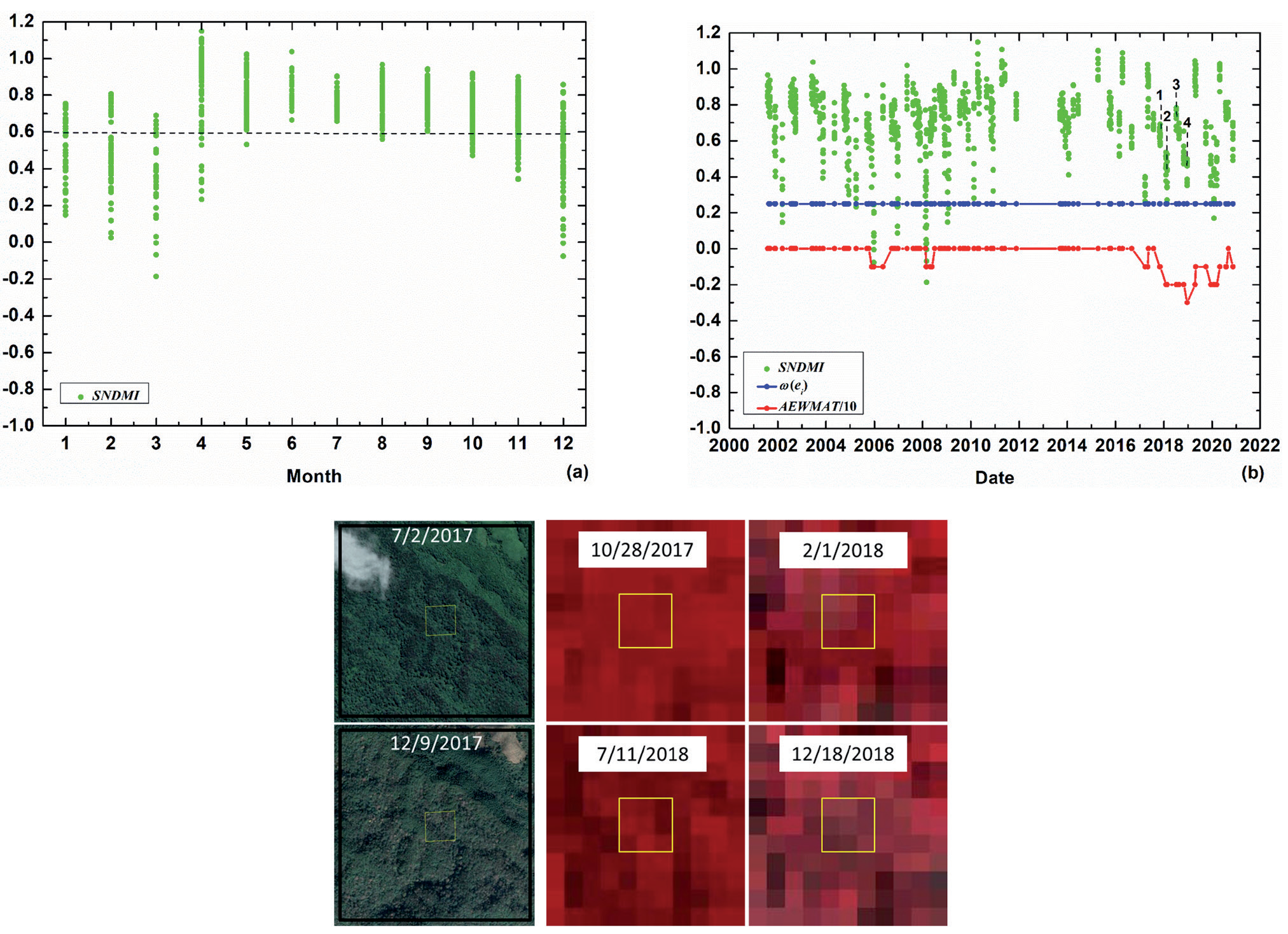
1) the consecutive noise and 2) the difference in forest seasonal variations. Consecutive noises that Fmask did not remove may be falsely detected as a disturbance. As shown in Fig. 7, consecutive shadows that appeared on October 31 and December 18, 2018 (second and third dash lines) resulted in three consecutive out-of-control signals (from third to fifth dash lines). Because of the inertia problem caused by the small value of the equivalent smoothing coefficient ω(ei), the AEWMAT values on the dates corresponding to the fourth and fifth dash lines were determined by historical values on the previous dates when shadows appeared, and then less than 0 even though shadows disappeared on the current two dates. Therefore, the AEWMATCD algorithm more easily mistakes consecutive (even less than three times) noise for disturbance. The difference of seasonal variations among mixed forests may result in spatially normalized index SNDMI largely deviating from 1, thereby generating a false alarm. As shown in the high-resolution images of Fig. 8, the seasonality of the forest within the patch with 3Í3 pixels or spatially normalized windows was visually different in different seasons. Every month for 20 years (from 2001 to 2020), the SNDMI of the forest within the patch deviated from 1 at different levels, especially from December to March (Fig. 8a)). Therefore, the large deviation of SNDMI caused by the difference in seasonality in these months generated a false positive (Fig. 8b)). One possible solution to this problem is to select the NDMI value of the forest pixels with the same tree species as the central pixel as the median NDMImedian according to the tree species classification map. However, it would make the algorithm complicated and time-consuming.
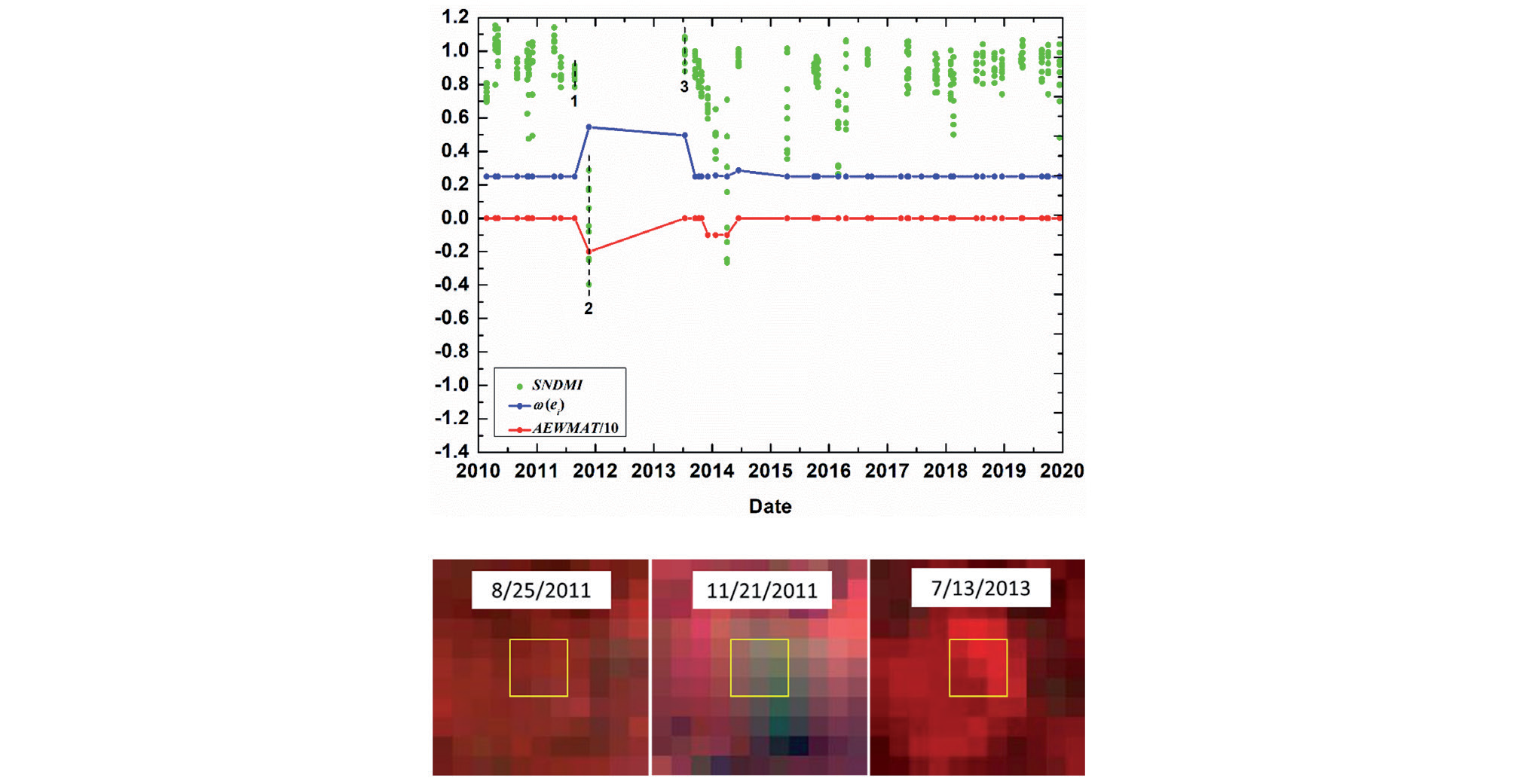
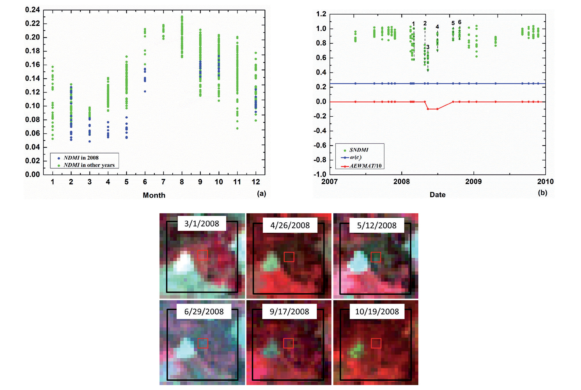
The omission error was mostly due to the following reasons: 1) excessively low disturbing signals; 2) the extremely sparse clear observations during disturbance; and 3) the relatively small spatially normalized window resulting in the covering up of disturbance with a wide range. Although the AEWMATCD algorithm can effectively detect disturbance agents with low-magnitude change, some disturbance agents (e.g., selective logging and insects) with excessively low disturbing signals are still hard to characterize. As shown in Fig. 9, insect agents lead to excessively subtle changes: the SNDMI median of the pixels within the patch drops from 0.79 at the previous time step before disturbance to 0.50 in the duration of disturbance (the black box), and the medians at each time step in the black box are between 0.40 and 0.61. Although the absolute value of the lower CL is small (-0.873), excessively low severity makes nearly all chart value AEWMA-ti cannot cross the lower CL, and only the last AEWMAT value in the duration of the disturbance is equal to -1. Extremely sparse clear observations would make disturbance hard to detect since the number of clear observations during disturbance is less than the requested number of consecutive signals for determining disturbance. As shown in Fig. 10, only one clear observation on the date corresponding to the second dash line recorded a disturbance due to the absence of clear observations in 2012 and a possible recovery in 2013. Therefore, the number (1) of out-of-control signals is below the requested number (3) of consecutive out-of-control signals for determining disturbances, resulting in omission error. When the spatial range of the disturbance agent is larger than the size of the spatially normalized window, the SNDMI of disturbed pixels is close to 1 because the forest pixels corresponding to NDMImedian are also disturbed. Then, it smoothed out the influence of disturbance. As shown in Fig. 11, the NDMI of forest patches from April to June in 2008 were generally lower than those in other years (Fig. 11a)). The SNDMI of disturbed pixels largely deviated from 1 when insect outbreaks occurred in the partial forest pixels within the spatially normalized window on April 26 and May 12, 2008 (second and third dash lines in Fig. 11b)). Then, the SNDMI of disturbed pixels is close to 1 when the insect occurred throughout the spatially normalized window on June 29 (fourth dash line in Fig. 11b)), followed by gradual and full recovery in September and October (fifth and sixth dash lines in Fig. 11b)). This resulted in the lack of three consecutive out-of-control signals for determining disturbance during the insect outbreaks. Therefore, to avoid such a situation, the proper size of the normalized window should be defined according to the extent of disturbance agents in the specific region.
Fig. 6.
Timely detection of high-magnitude disturbance agent (clearcut) within a 3×3 spatial window (yellow boxes) using AEWMATCD algorithm a) and omission error in detection using EWMATCD algorithm with a fixed small value of λ(b): sparse clear observations during disturbance and inertia problem of EWMA-t chart. The dates corresponding to six dashed lines in the charts correspond to those of Landsat images in turn.
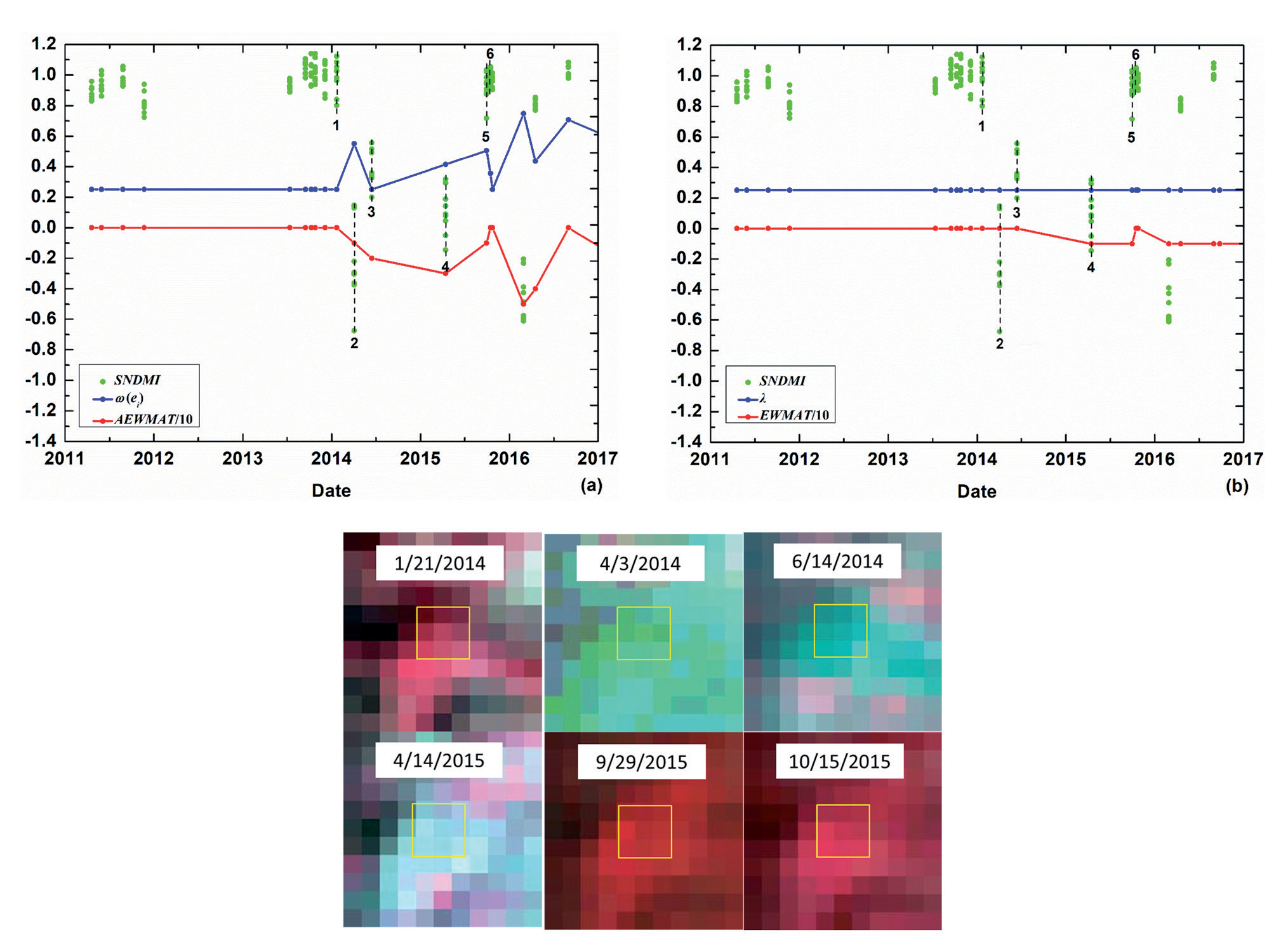
Table 1.
Spatial accuracy assessment of diverse disturbances detection.
Assessment of Disturbance Detection Accuracy in the Temporal Domain
Given that Landsat time series are sparse, the date corresponding to the first image in which disturbance was identified through visual interpretation was treated as the initial occurrence date. Then, the temporal accuracies of the 308 reference disturbed samples detected by the AEWMATCD algorithm were further assessed (Table 2). 78.9% of disturbed samples were detected by the AEWMATCD algorithm on the initial date of disturbance (same time step). If a one time step delay (late = 1 time step) in detecting disturbances is acceptable, 89.3% (78.9%+10.4%) of disturbance samples were correctly signaled within two time steps after disturbance occurrences, showing a rapid response of the AEWMATCD algorithm to disturbances.
Fig. 8.
Commission error of detecting disturbance agent within a 3×3 spatial window (yellow boxes) using AEWMATCD algorithm: difference of forest seasonal variations. a) SNDMI of forest patch with the 3×3 spatial window in every month of 20 years (from 2001 to 2020); b) AEWMA-t chart. The dates corresponding to four dashed lines in AEWMA-t chart correspond to those of Landsat images in turn, and the black boxes in the high-resolution images represent the spatially normalized window.
Considering each disturbance type (Table 2), 84.2% of clearcut were detected by the AEWMATCD algorithm on the initial date of disturbance and followed by fire (81.1%), meaning the timely response of AEWMATCD algorithm to high-magnitude disturbances. The comparison of different disturbance agents showed that detecting clearcut and fire with high magnitude on the same time step was earlier and more timely than selective logging (56.3%) and insects (50.0%) with low magnitude. The reason is that the change severity and equivalent smoothing coefficient ω(ei) of high-magnitude disturbances are both higher than those of low-magnitude disturbances, resulting in quicker detection of the high-magnitude disturbances. However, 71.9% (56.3%+15.6%) of selective logging and 75.0% (55.0%+20.0%) of insects were still correctly signaled within two time steps after disturbance occurrence, showing moderate success for low-magnitude disturbance detection and the potential for early warning.
For further verifying whether the AEWMATCD algorithm effectively overcomes the inertia problem, the EWMATCD algorithm with a fixed small value of λ = 0.25 was executed on 308 reference disturbed samples detected by the AEWMATCD algorithm. As shown in Table 2, regardless of whether it is the same time step or within two time steps, the temporal accuracies (58.8% or 58.8%+16.5% = 75.3%) of disturbed samples detected by the EWMATCD algorithm are both lower than those (78.9% or 89.3%) detected by the AEWMATCD algorithm. More seriously, several disturbed samples (5.8%) were undetected by the EWMATCD algorithm because of sparse, clear observations during the disturbance and inertia problem of the EWMA-t chart (Fig. 6b)). For high-magnitude disturbances, due to the adaptive adjustment of the equivalent smoothing coefficient ω(ei), the temporal accuracies of both clearcut and fire detected on the initial occurrence date are raised by more than 20% using the AEWMATCD algorithm, compared with the EWMATCD algorithm. For low-magnitude disturbances, the temporal accuracies of both selective logging and insects detected on the initial occurrence date using the AEWMATCD algorithm are basically the same as those using the EWMATCD algorithm. The reason is that ω(ei) in the AEWMATCD algorithm generally keeps its initial small value of 0.25 due to the low severity of selective logging and insects, which is the same as the fixed small value of λ in the EWMATCD algorithm. These results further indicated that the AEWMATCD algorithm could effectively solve the inertia problem and temporal delay of high-magnitude disturbance detection.
Fig. 9.
Omission error of detecting disturbance agent (insects) using the AEWMATCD algorithm: excessively low disturbing signals. The black box represents the duration of disturbance.
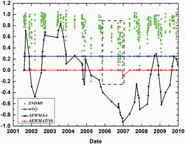
Fig. 10.
Omission error of detecting disturbance agent (clearcut) within a 3×3 spatial window (yellow boxes) using the AEWMATCD algorithm: the extremely sparse clear observations during disturbance. The dates corresponding to three dashed lines in AEWMA-t chart correspond to those of Landsat images in turn.
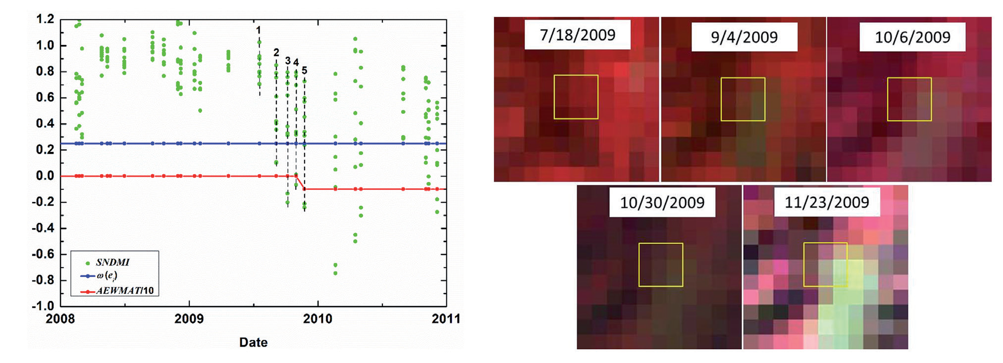
The temporal errors of the AEWMATCD algorithm are mainly due to low-magnitude disturbances initially occurring in partial pixels, resulting in excessively low disturbing signals (AEWMA-ti) at the first few time steps. This makes the AEWMATCD algorithm unable to detect the disturbance until the disturbing signals are accumulated and amplified. Fig. 12 shows selective logging started to occur in the partial pixels (5/9) of the 3Í3 spatial window on September 4, 2009 (corresponding to the second dash line in the AEWMA-t chart). This leads to the relatively low absolute values of the current Ti and chart value AEWMA-ti that cannot cross the lower CL in a timely manner. As selective logging occurred in the rest of the pixels and even clearcut occurred in the partial pixels, the accumulated disturbing signal (AEWMA-ti) was gradually enhanced. It became large enough to identify the disturbance on November 23, 2009 (fifth dash line in the AEWMA-t chart), resulting in a temporal delay of three time steps.
Fig. 11.
Omission error of detecting disturbance agent (insects) within a 3×3 spatial window (red boxes) using AEWMATCD algorithm: the relatively small size of spatially normalized window resulting in the covering up of disturbance with a wide range. a) NDMI of forest patch with the 3×3 spatial window under insects stress in 2008 and other years; b) Insects detection using AEWMA-t chart. The dates corresponding to six dashed lines in AEWMA-t chart correspond to those of Landsat images in turn, and the black boxes are the spatially normalized windows.
Discussion
Through setting the initial small value of ω(ei) to make the CL (disturbance threshold) low for effectively detecting the low-magnitude disturbances and adaptively tgetting ω(ei) larger for overcoming the inertia problem of high-magnitude disturbance detection, the proposed AEWMATCD algorithm can detect both low- and high-magnitude disturbances. However, a smaller value of ω(ei) is not always better. Although the smaller ω(ei) makes the CL lower and may reduce the omission errors of low-magnitude disturbances, it also may increase the commission errors resulting from the difference in forest seasonal variations or noises (Figs. 7 and 8). Meanwhile, the smaller ω(ei) further lowers the temporal accuracy of low-magnitude disturbance detection, even resulting in omission errors due to the extremely sparse clear observations during disturbance (Fig. 10). Therefore, setting the reasonable initial value of ω(ei) in the proposed AEWMATCD algorithm is important.
Table 2.
Temporal accuracy assessment of diverse disturbances detection.
Fig. 12.
Temporal delay of detecting disturbance agent (selective logging) within a 3×3 spatial window (yellow boxes) using AEWMATCD algorithm: low-magnitude disturbance initially occurred in partial pixels. The dates corresponding to five dashed lines in AEWMA-t chart correspond to those of Landsat images in turn.
In this study, the proposed method detects diverse disturbance agents using a single spectral index. However, the responses of different spectral indices to different disturbance agents, and even to the same ones, are different [46, 54]. Bueno et al. [46] found a low rate of spatial agreement among disturbance maps separately produced by seven spectral indices. Compared with detection relying on a single spectral index, a multispectral ensemble for disturbance detection might enhance the ability to reduce false and omission errors. The ensemble rules mainly include two types: one that uses simple combination rules such as an average, majority, or special distribution [20, 29, 55, 56] and another that uses classification rules such as the random forests model [54, 55, 57-59]. In future studies, it is worth improving the proposed algorithm to detect forest disturbances using multiple spectral indices.
Disturbances cause changes in both forest spectral and spatial features, and therefore, forest disturbance agents can be comprehensively described from temporal, spatial, and spectral dimensions, which can reduce the commission and omission errors in change detection. Some studies have explored forest disturbance detection by integrating spatio-spectral change information, such as change detection using spatial feature time series[60-63], object-oriented change detection [64, 65], and false positive elimination based on spatial correlation of disturbance agents [27, 54]. Although this study integrates spatial context in spatial normalization of NDMI, spatio-temporal autoregressive regression using SEM model, and the spatial statistic Ti, spatial features change caused by disturbance, was not directly used to enhance the change signal for disturbance detection. Future research could focus on disturbance detection by integrating spectral and spatial information.
By lowering the temporal delay of the inertia problem, the proposed AEWMATCD algorithm reduces omission errors in areas with sparse time series. However, short-term disturbance agents, such as reforestation post-deforestation or seasonal diseases and insects, may still be omitted when the disturbance agent wasn’t continuously observed during the excessive temporal gaps in sparse Landsat time series. Meanwhile, timely detection of disturbance agents that may finally result in a stand-replacing transition as an early warning is also critical for forest management [22, 25, 27, 66, 67]. Recently, the framework of integrating multi-sensor datasets into a continuous observation set to build a dense dataset as the input of change detection algorithm provides an opportunity for timely capturing both short- and long-term disturbance agents [8, 15, 68, 69]. For example, Cardille et al. [15] fused Landsat 8 and Sentinel-2 data streams to detect forest disturbances with reduced latency. Thus, densifying the time series through integrating observations from compatible satellite platforms provides an alternative for lowering omission errors and early detection, which is worth exploring in future research.
Accurately identifying the attribution of disturbances is crucial for formulating effective management strategies. This paper primarily focuses on detecting various forest disturbances of different intensities, while future research will further expand into the field of disturbance attribution. We will utilize change detection followed by classification methods (such as combining supervised classification to further differentiate forest disturbance types based on disturbances detection) or direct classification methods (such as directly detecting types of disturbances using multi-temporal remote sensing imagery). This approach will enable the precise identification of different types of disturbances, allowing for more targeted management and response measures to protect the health and stability of forest ecosystems.
At the same time, to address the issues of small sample sizes and sample imbalance in disturbance attribution, we will explore the use of deep learning methods to enhance model performance. Generative models, such as Generative Adversarial Networks (GAN) and diffusion models, can effectively generate synthetic samples, expanding the training dataset and improving model robustness. Additionally, we will consider using a mutual guidance framework based on confidence learning, leveraging the interaction between multiple models to fully utilize unlabeled data and enhance the diversity of training data. The combination of these methods is expected to significantly improve the ability to identify different types of forest disturbances.
In practical applications, the AEWMATCD algorithm can significantly support forest management. In the future, this method can be applied in various geographical locations and climate types. The algorithm can be used to monitor disturbances such as forest pests and diseases, wildfires, or illegal logging, helping managers make quick decisions. For example, against the backdrop of escalating global warming, forest ecosystems in regions like the Amazon rainforest and the Tibetan Plateau are facing greater pressures. By applying the AEWMATCD algorithm, managers can promptly detect disturbances in these areas and take proactive protective measures.
Conclusions
Detection of diverse disturbance agents is the precondition for attributing diverse forest disturbances. However, most change detection algorithms were designed to detect specific disturbance agents, which may not be the most effective way to describe all disturbance agents with different change magnitudes. Meanwhile, these algorithms using dense time series are inapplicable in frequent cloud cover regions. The AEWMATCD algorithm is proposed to address these issues, using sparse Landsat time series to detect diverse forest disturbances with different change magnitudes. Based on the EWMA-t chart that is sensitive to low-magnitude disturbances and designed for sparse observations, an adaptive strategy that adaptively adjusts weights ω(ei) of historical chart value and current residual statistics in the chart is introduced to EWMA-t chart (AEWMA-t): when low-magnitude disturbances occurred, current AEWMA-t chart value can exceed the low control limits determined by an initial small value of ω(ei); conversely, more weight was assigned to a current residual statistic with a high negative value for quickly detecting high-magnitude disturbances. The AEWMATCD algorithm effectively detects both low- and high-magnitude disturbances based on the adaptive adjustment of the smoothing coefficient ω(ei) to different change magnitudes. It possesses the ability to detect disturbances in regions with insufficient data by integrating temporal-spatial contexts. Detection accuracies in both spatial and temporal domains of high-magnitude disturbances are higher than those of low-magnitude disturbances. It showed a rapid response of the AEWMATCD algorithm to high-magnitude disturbances, and the moderate success of low-magnitude disturbances detection proved the potentiality for early warning. The proposed AEWMATCD algorithm presents an alternative for quickly and accurately capturing diverse forest disturbance agents driven by natural causes and human activities in regions with insufficient data, laying the foundation for subsequent attribution of forest disturbance agents.

