

Introduction
Obtaining the geostatistics of soil samples can help government departments and agencies to accomplish soil surveys, but is always affected by the spatial heterogeneity caused by anthropogenic influences such as mining, soil covering, soil improvement, etc. [1–4]. Previous studies on anthropogenic soil related to mining have often focused on issues of environmental significance [5, 6]. China has recognized the importance of protecting the soil environment and has implemented the Action Plan for Prevention and Control of Soil Pollution [7]. In addition, the risk screening and intervention values for soil contamination have been confirmed through soil environmental quality risk control standards, which also guide the monitoring of land consolidation areas [8].
Both the environmental factors and physicochemical properties of soil exhibit spatial heterogeneity and autocorrelation, and a semi-variable function has always been used as the spatial model before obtaining a locally linear unbiased estimation [9, 10]. However, the modeling data, which may be either raw data or Box-Cox conversion data, need to have or approximate a Gaussian distribution. Moreover, owing to the random effects or extremal distribution, the spatial heterogeneity and unbiased estimation obtained from semi-variance do not perform well enough. For instance, researchers have proposed multifractal analysis to manage the geochemical anomalies at the boundaries between different geologic zones [11, 12]. In addition, Wang et al. developed the sandwich model for stratified mapping in scenarios in which spatial heterogeneity relies more on the spatial stratification of some influencing factors [13, 14]. For semi-variance based on stratification heterogeneity, it is difficult to fit a function due to the cross-distribution of the stratifications and the limited number of samples. Compared with the Gaussian unbiased estimation, which reduces the spatial correlation of the extremes, the copula-based spatial model may be sufficient and provide more characterization of the spatial variations in the heavy metal concentrations of the soil [15–18]. Bárdossy (2006) first proposed the use of the copula-based spatial model as a replacement for variograms and covariance functions in order to describe the spatial heterogeneity. The structure of the copula-based spatial model is composed of the dependent function and the marginal distributions; and the dependent function, i.e., the copula, is the basis, which is based on Sklar’s theory [19, 20]. Some experts have used the Copula-based model to study the spatial dependence of extreme rainfall weather in the Mediterranean Sea, and there are also studies that use the spatial copula model combined with Bayesian approximation to predict extreme temperature [16, 17]. In addition, the copula has many families that can serve as alternatives for spatial model construction [21, 22], which can achieve visualization through the web app Copulatheque [23].
Soil pollution should be investigated before and after land consolidation in mining areas to identify and control the key environmental areas [24–27], especially when a certain emergency threshold may have been exceeded [28]. Although a spatial Bayesian process unifies the estimation and prediction and takes into account the uncertainties of the model parameters, which means it can acquire the uncertain information in the high-risk areas regarding heavy metals, it generally assumes that the model is a Gaussian random field [29, 30]. In addition, it is possible to use indicator kriging (IK), which does not require the data to obey the normal distribution. As a non-parametric geostatistical method, IK is robust regarding outliers [9, 31, 32]. However, one threshold means one model with one map, which is extremely unintelligent. Thus, a copula-based spatial model can provide the probability distribution function of each prediction site and can identify the extremal regions, i.e., where the heavy metal concentrations of the soil exceed particular thresholds with a 50% probability [33]. It can be concluded that the copula-based spatial model combines the optimal prediction results of the Bayesian spatial model and the non-normality assumption of IK.
In summary, we analyzed and predicted the spatial heterogeneity of the As, Cd, Cr, Hg, and Ni contents and pH value of soil in a mine consolidation area, and we identified the extremal regions of Cd pollution of the soil. First, using variogram analysis and a geographic detector, the spatial heterogeneities of these environmental factors were determined. Second, the copula-based and Gaussian spatial models were compared, and the soil environmental factors were predicted throughout the area. Finally, the extremal regions were identified using the copula-based spatial model and the Gaussian spatial model through a Bayesian process.
Materials and Methods
Study Area
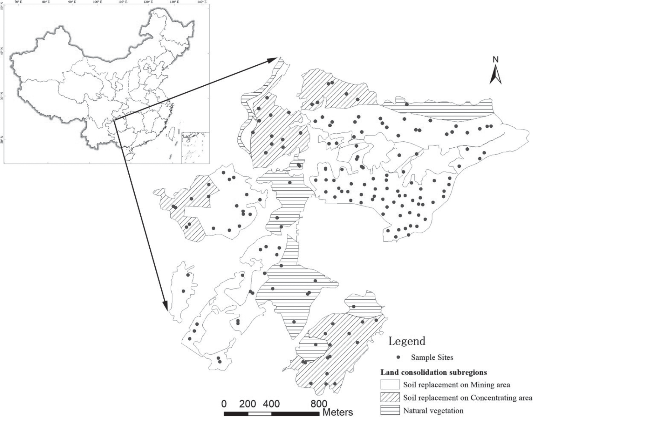
The study area is located in the southern Sichuan Basin (27°41′–28°20′ N, 105°34′–106°20′ E), which has a long history of sulfur ore mining. It shares the climatic characteristics of both the Sichuan Basin and the Guizhou Plateau and is located in the subtropical humid climate zone, with mean temperature, precipitation, and relative humidity values of 16.8–18.6°C, 1000 mm, and 83%, respectively. The elevation of the study area ranges from 501 m in the southwest to 948 m in the northeast, and the main soil types are yellow soil and brunisolic soil. Owing to long-term mining and concentration, most of the study area contains harmful substances, such as sulfur waste, and the original ecological landscape has been seriously damaged. Since 2013, consolidation of abandoned industrial and mining areas has been conducted, including soil replacement in mining areas (SRM), soil replacement in concentration areas (SRC), and natural vegetation.
Sampling and Analyses
The soil environment survey for heavy metals included 175 observations throughout the entire 4 km2 study area. The distribution of all of the samples is shown in Fig. 1. The soil samples were collected from the topsoil layer (0–20 cm), and they were combined into a composite sample for a 20×20 m area. The soil samples were air-dried, sieved to 2 mm, and digested using HNO3 and H2O2 via Method 3050B (USEPA, 1996). The Cd, Ni, and Cr concentrations of the digestion solution were measured via inductively coupled plasma optical emission spectrometry (ICP-OES, Optima 5300DV, PerkinElmer Instrument Co., Ltd., USA), and the As and Hg concentrations were analyzed using an atomic fluorescence spectrometer (AFS- 2202, Haiguang Instrument Co., Ltd., China). The pH values of the soils were determined using the potentiometric method. Standard reference soils GSS-1 and GSS-2 were obtained from the Center of National Standard Reference Material of China and were used for quality assurance and quality control.
Stratification of Spatial Heterogeneity Using the Geographic Detector
The geographic detector is a geostatistical method that can be used to explore spatial heterogeneity without the Gaussian distribution assumption. Its core idea is that if the environmental factor is dependent on one influencing factor, they may have similar spatial distributions [34, 35]. The goal of this study was to identify the environmental factors with significant spatial differences due to anthropogenic influences, which always exhibit intense randomness. In addition, the geographic detector provides the driver of environmental pollution to a certain extent. Here, we used the q value of the geographic detector:
where s = 1, …, L is the stratification of the influencing factors; Ns and N are the number of units in each stratification and in the entire district, respectively; and σ2s and σ2 are the variances in each stratification and in the entire district, respectively.
Geostatistical Models
Gaussian Spatial Models and Bayesian Process
The Bayesian spatial model is a Gaussian spatial process, which fits the multivariate normal distribution, and the basic function, which is obtained from the semi-variogram is
where μ(x) = m is constant; the spatial effect ω(x) = f(σ2, φ) is a function of the partial sill (σ2) and the range (φ); and non-spatial effect ε(x) = f(τ2) is a function of the nugget (τ2).
The procedures of the Bayesian spatial model include establishing the model and the prior distribution, the posterior distribution based on Markov Monte Carlo (MCMC) sampling, and the spatial prediction based on the posterior distribution [36, 37].
First, based on the Bayesian hierarchical modeling approach, its data model, procedural model, and parametric model are
where MND is the multivariate Gaussian distribution function; H(φ) is the correlation matrix, which is represented by an exponential function, i.e., H(φ) = exp(-φ||xi – xj||), and ||xi – xj|| is the distance between two spatial points; m, σ2, φ and τ2 are random variables, which are independent with each other; m is constant; and the three other variables have exponential prior distributions.
Then, the posterior distribution sampling is conducted using the Markov chain Monte Carlo (MCMC) method, with the convergence of the Geweke z value. The mathematical formula is
where J0(θ) is the prior joint probability distribution of the four parameters m, σ2, φ and τ2, and f(Z|θ) is the likelihood of the maximum likelihood estimation.
Finally, the spatial prediction is realized using the following equation:
In this study, the R package spBayes and the sp and geoR packages were used to obtain the Bayesian spatial prediction of the soil environmental factors [38]. The Metropolis algorithm was used in the MCMC, with 10000 iterations and Geweke z value convergence checking.
Copula-Based Geostatistical Models
The copula-based spatial model describes the spatial stochastic field based on Sklar’s theory [28, 39, 40]. The basic formula is
where Cθ,λ is the n-dimensional copula, with a correlation structure related to θ and λ; and Fη is the marginal distribution function related to η.
The sort order of the marginal functions does not affect the results because the copula is symmetric, which means that the sort order of the observations does not affect the structure of the spatial model. Similar to the traditional method, two points far apart are known to have mutual independence, while there is a strong dependency between points close to each other. In this study, the Gaussian spatial copula with non-Gaussian margins was used for the soil environmental factors, and the maximum likelihood function estimation through Θ = (θ, λ, η) was as follows:
where cθ,λ is the probability density function of the copula; and D = {z1,…, zn} are the observations.
Based on the observations and parameter estimation, the probability density distribution at location needs to be predicted as follows:
where cθ,λ is the probability density function of the conditional copula. The expected value and variance are calculated respectively as follows:
It should be noted that the direct calculation of the multivariant copula is miscellaneous and has poor accuracy, so the multivariant probability density function was decomposed into a series of copula pairs and marginal functions using the vine-copula method. In this study, the C-Vine copula model was used [41, 42]. In this study, the spcopula and VineCopula R packages were mainly used to create the copula-based spatial model [15, 40, 43].
Validation of the Spatial Prediction Effect
In this study, first, the validation of the spatial prediction effect of the expected values for both the copula-based and Gaussian spatial models was conducted, and then, the comparison of the extremum characteristics was conducted [44, 45]. The performances of these models were compared via leave-one-out cross-validation, which was utilized to calculate the mean absolute percentage error (MAPE) and the goodness fit (R2). For each observation site xi, the distribution of Zi was conditional upon all of the observed data, except when z(xi) was calculated and the predicted probability that z < z(xi) was extracted. The cross-validation MAPE and R2 were computed as follows:
where Z^–i(xi) is the prediction at the location xi calculated using all of the observed values, except z(xi); z–(xi) is the mean of z(xi). The closer MAPE is to zero, the better it is; and, an R2 value closer to 1 is better.
The extremum analysis of the copula-based and Bayesian spatial models was based on the distribution of the probability of the predicted locations in order to obtain the extremal regions [18]. First, the observations exceeding the specific threshold were identified. Then, the predicted regions exceeding the threshold with a 50% or 75% probability were identified, and the coverage of the observations was checked.
Results and Discussion
Descriptive Statistics and Variogram Analysis
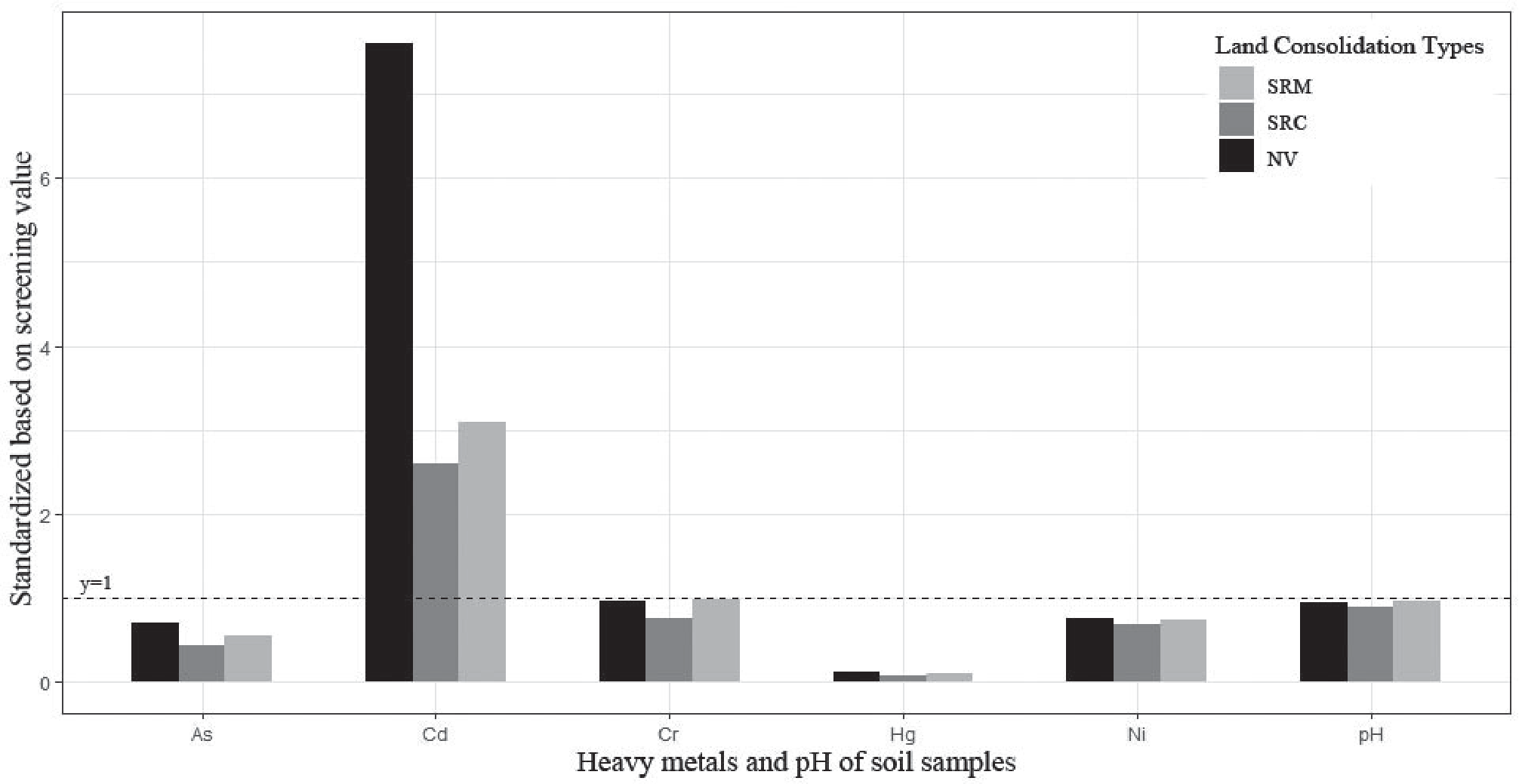
The descriptive statistics of the heavy metal concentrations and pH values of the topsoil in the mining area after consolidation are presented in Table 1. The As, Cd, Cr, Hg, and Ni concentrations and pH values of the soil throughout the study area were 4.19–32.92 mg·kg−1, 0.09–6.29 mg·kg−1, 95.26–556.53 mg·kg−1, 0.03–0.47 mg·kg−1, 21.19–166.89 mg·kg−1, and 2.78–8.52 mg·kg−1, respectively. Based on the soil screening values (SVs), the Cd concentrations of the soil seriously exceeded the regulation standard, and the mean concentrations of the other heavy metals were all below the SVs. According to the coefficients of variation (CVs) for the heavy metals, there was considerable variation within the range of 31.17% to 83.72%, and the CVs of the pH had the lowest value. After standardization using the SVs, Fig. 2 shows whether the concentrations of the heavy metals in the three consolidation types exceeded the regulatory limit. It shows that the standardized Cd value is much greater for the natural vegetation than for the SRM and SRC, while the values for the other heavy metals are similar for the different consolidation types.
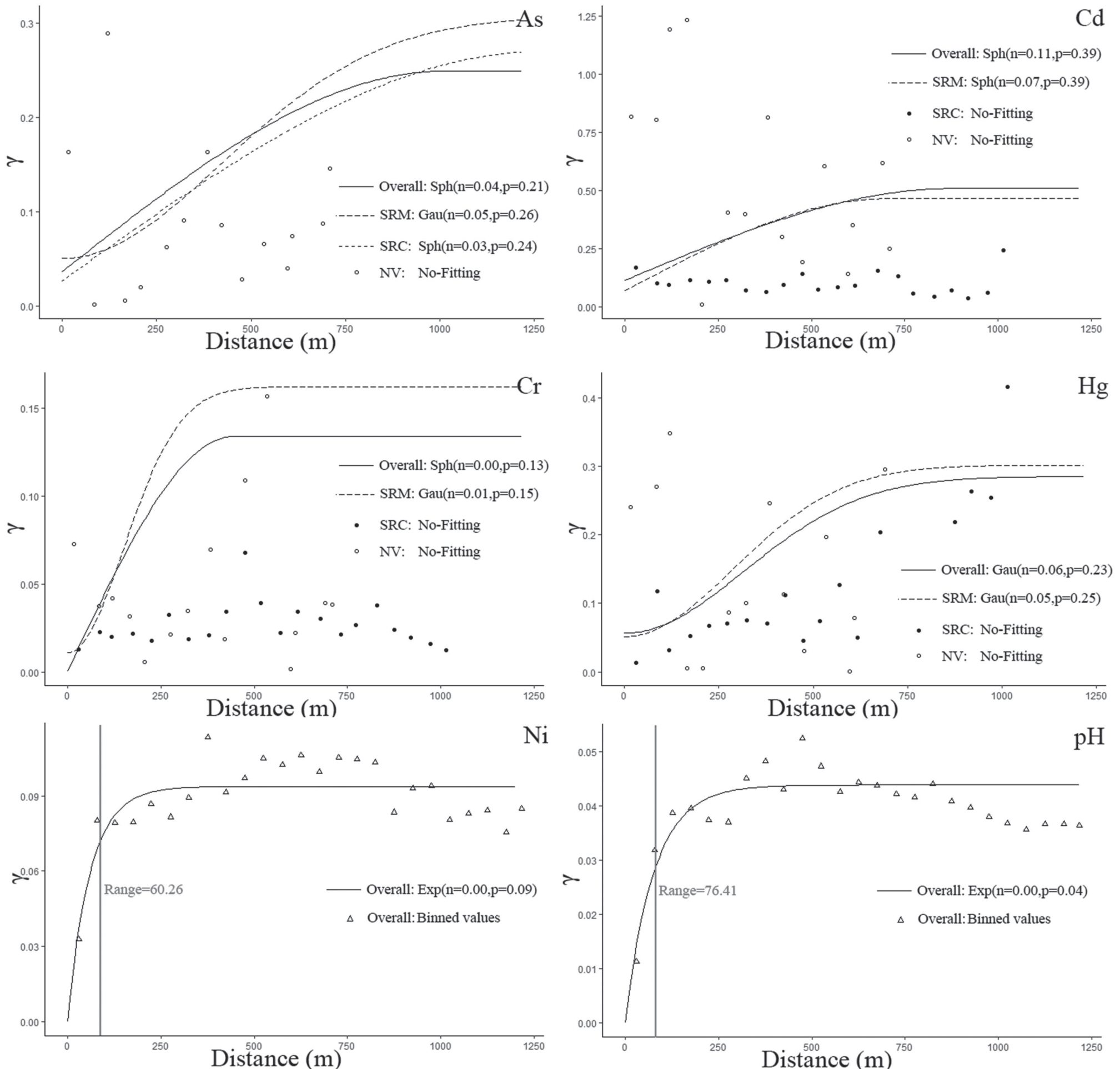
The variogram analysis of the heavy metal concentrations and pH values of the soil based on their spatial distributions is presented in Fig. 3. Fig. 3 shows that the variograms for As, Cd, and Hg hold for a large distance (at least 600 m) based on the spatial autocorrelation. Cr has a range of 385.72 m, while those of Ni and pH are 60.26 m and 76.41 m, respectively. Several studies have suggested that the nugget/ sill ratio n/(n+p) represents the ratio of the spatial heterogeneity, which obtains the spatial heterogeneity from the randomness of the variable, while the 1−n/(n+p) value reflects the structural spatial heterogeneity [31, 46, 47]. Thus, this range can be considered to be the spatial heterogeneity scale, and the larger the nugget/sill ratio is, the stronger the random spatial heterogeneity is. A ratio of greater than 75% indicates strong random spatial heterogeneity; values of 25–75% indicate moderate random spatial heterogeneity; and values of < 25% indicate weak random spatial heterogeneity. Overall, in the study area, the nugget/sill ratios of As, Cd, Cr, and Hg were 16.00%, 22.00%, 0%, and 20.69%, respectively, and in the different types of consolidation land, the ratios also indicate weak random spatial heterogeneity. Moreover, Ni and pH also exhibited weak random spatial heterogeneity.
Based on the first law of geography, Cr, Ni, and pH exhibited very weak random spatial heterogeneity, which was calculated from the variograms. Weak random spatial heterogeneity is equivalent to strong autocorrelation. The emergence of this situation can be attributed to the soil replacement in most regions of the study area. However, the spatial heterogeneity of As, Cd, and Hg are somewhat different, including a larger range and stronger random spatial heterogeneity. Thus, we conclude that several influencing factors continue to affect the spatial distributions of the As, Cd, and Hg concentrations.
Table 1.
Descriptive statistics of heavy metal concentrations and pH values of the soil samples.
Validation of the Performances of the Spatial Prediction Models
Similar to the above variogram analysis, for the copula-based spatial model, a correlation function related to the spatial distance also needs to be established. In this study, the rank correlation for each bin was calculated, which was obtained from the point pairs in each step, to generate a function through polynomial regression (Fig. 4). Similarly, Ni and pH also had shorter ranges regarding their spatial heterogeneity, and the strengths of the correlations for As, Cd, Cr, and Hg gradually decreased as the distance increased, with good fitting conditions. However, their fitting functions could not be used to build an indicator similar to the nugget/sill ratio, so we explored the stratification of the spatial heterogeneity based on the different land consolidation types using a geographic detector. The geographic detector analysis generated q values (Table 2), and the larger the q value is, the stronger the stratified spatial heterogeneity is. It was found that the q value of Cd was the largest and it was extremely significant, which means the spatial distribution of Cd was highly dependent on the consolidation type. In addition, the q value of As was significant, while those of the others were not significant. Thus, the spatial distribution of Cd had a strong stratified spatial heterogeneity, and As had a moderate stratified spatial heterogeneity. However, based on the variogram analysis, the distributions of all of the heavy metals exhibited weak random spatial heterogeneity. Based on previous studies [34, 35], we conclude that the stratified spatial heterogeneity is not affected by the random spatial heterogeneity. Moreover, the former relies on spatial stratification, while the latter relies on samples, which means that they are calculated using different geostatistical scales but are complementary in terms of exploring spatial heterogeneity.
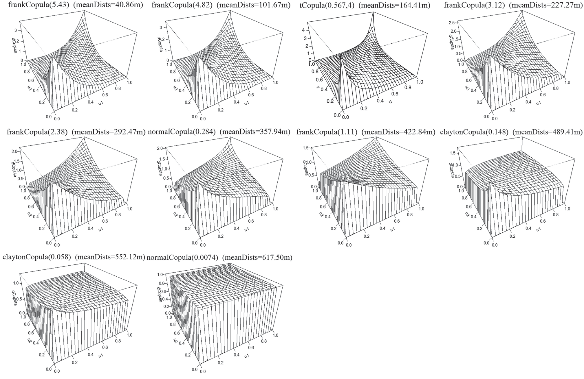
The copula-based spatial model constructs the different copulas based on the marginal distribution of the observations in each step. Cd is discussed as an example (Fig. 5). Because the joint probability distribution is only related to the distance between the spatial points, all of the copulas are symmetric. There are four types of copulas, including the frankCopula, tCopula, normalCopula, and claytonCopula. The selection of these copulas and their parameters is determined via maximum likelihood estimation. The two-dimensional frankCopula and claytonCopula are both Archimedean copulas with a single parameter [48–50]. The frankCopula is characterized by the symmetry of the upper and lower tails, while the claytonCopula is characterized by a light upper tail and heavy lower tail. The frankCopulas of Cd are located at mean distances of 40.86 m, 101.67 m, 227.27 m, and 422.84 m. In addition, as the parameter decreases from 5.43 to 2.38, the tails of the frankCopulas become lighter, which indicates stronger randomness throughout the probability distribution. The claytonCopulas of Cd are located at mean distances of 489.41 and 552.12 m, and as the parameter decreases from 0.148 to 0.058, the lower tails become lighter. The upper and lower tails of the normalCopula are also symmetrically distributed. Compared with the other symmetrical copulas, the tCopula always has heavy upper and lower tails. When the tails of the copulas with mean distances of greater than 227.27 m become light, the tCopula with a mean distance of 164.41 m has the heaviest tail, which means that the extremal regions appear within a radius of nearly 200 m around the extreme samples with a high probability.
Fig. 3.
Variogram analysis throughout the study area and for the different land consolidation types (Note: n stands for nugget and p stands for partial sill, which were calculated from the variogram model, including spherical (Sph), exponential (Exp), and Gaussian (Gau). No-fitting indicates that no variogram function can be fitted to the specific data).
As was previously discussed, the copula-based spatial model does not have an indicator similar to the ratio of the heterogeneity from the variogram. The random error of the variogram fitting is finally summed up as the nugget, but the copula-based spatial model distributes the randomness to every copula in the form of probability through maximum likelihood estimation. Thus, the predicted results exhibit the characteristic of raw data rather than a Gaussian distribution.
After establishing the variogram, the Gaussian spatial model was used to conduct a locally optimal unbiased estimation for the predicted locations. If the raw data did not have a Gaussian distribution, a logarithmic or Box-Cox transformation was used. However, the copula-based spatial model does not require the data to obey a Gaussian distribution. The cross-validation of the spatial predictions obtained using both the Gaussian and copula-based spatial models is presented in Table 2. It reveals that the MAPE values of Cr, Ni, and pH, for both the Gaussian and copula-based spatial models, are much smaller than those of the other factors. This could be due to the weak random spatial heterogeneity of these three factors. In addition, the R2 value of Cr is the largest, which may be because it has the largest range among these three factors, which means more useful data for the local estimation of the locations. In general, the prediction effects of both models are very similar for Cr, Ni, and pH. In addition, the prediction of Cd based on the Gaussian spatial model has the largest MAPE value, which is largely because it has the greatest random spatial heterogeneity. However, among these heavy metals, Cd’s prediction effect was the most improved through the use of the copula-based spatial model, that is, its MAPE decreased from 0.33 to 0.29 and its R2 increased from 0.36 to 0.42. Moreover, the prediction of As was also improved through the use of the copula-based spatial model. Relative to the MAPE and R2 of the Gaussian spatial model, the improvements for Cr, Hg, and Ni were 5.88% (MAPE of Cr decreased from 0.17 to 0.16) and 3.92% (R2 of Hg increased from 0.51 to 0.53) at most, respectively. However, the improvements of Cd’s MAPE and R2 values were 12.12% and 16.67%, respectively, which are far better than those of the other heavy metals. In conclusion, the soil environmental factors of the consolidation land always exhibited weak random spatial heterogeneity because of the soil replacement in most of the study area, and the spatial model based on the Gaussian assumption satisfied the prediction requirements. However, some factors, such as Cd and As, in the study area may have strong stratified spatial heterogeneity, and their prediction effects were improved using the copula-based spatial model.
Fig. 4.
Strengths of the correlation functions calculated from the optimally estimated copulas per lag.
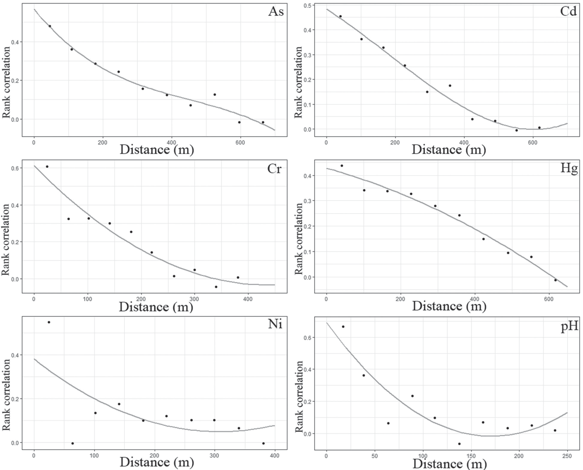
Table 2.
Performances of the different spatial models based on different q values from the geo-detector.
Identification of Extremal Regions for Heavy Metal Concentrations of the Soil
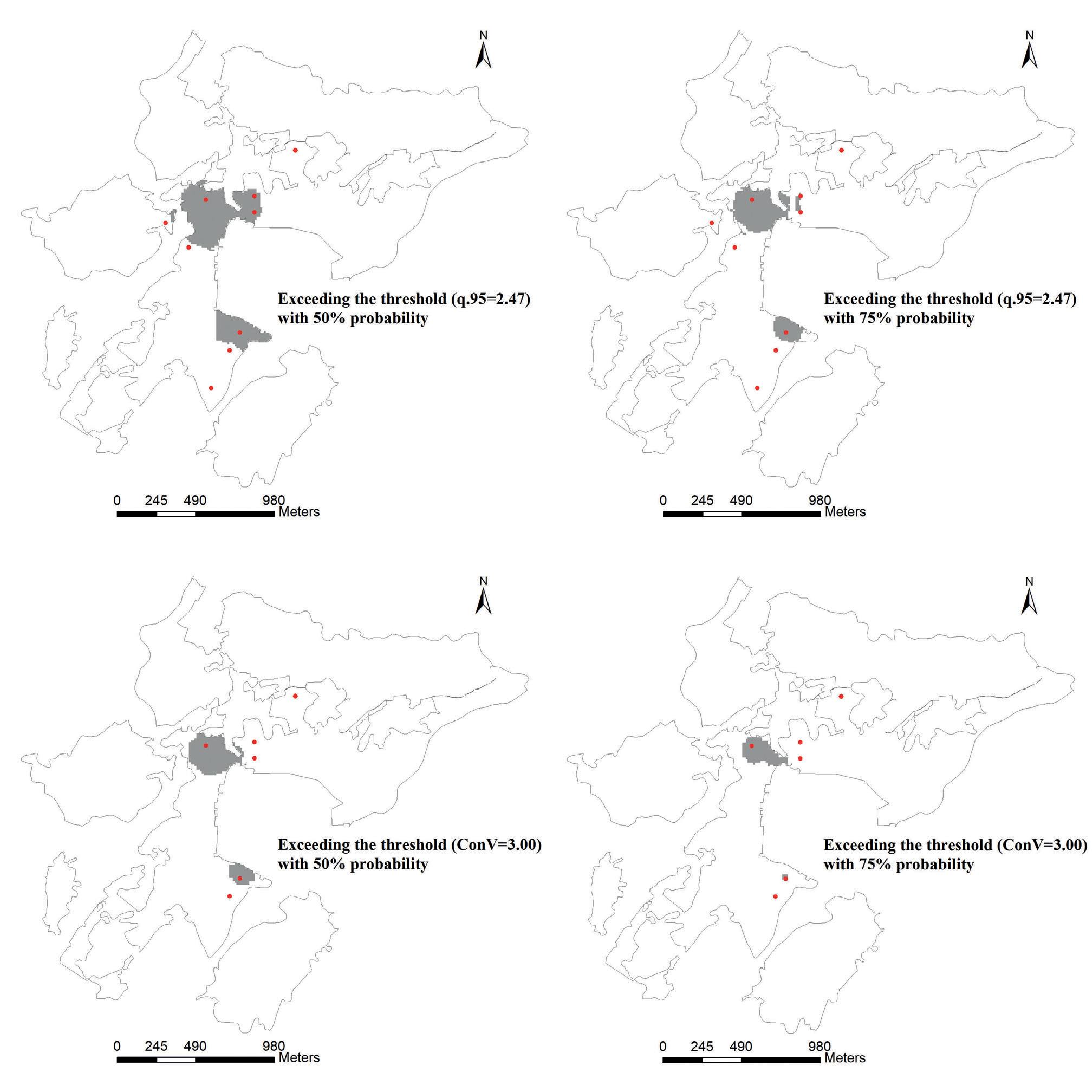
The prediction results obtained using the copula-based spatial model are the probability distribution for each location, so the Gaussian spatial model using the Bayesian process was used for comparison. In addition, the phenomenon of the Cd concentration of the soil in the study area exceeding the standard overwhelming occurred, so Cd was taken as the object of the extremal region identification study. Based on both observation statistics and regulation, two thresholds were set, including the 95% quantile of the samples (2.47 mg/kg) and the risk control value based on the regulation (3.00 mg/kg). These values are abbreviated as q.95 and ConV, respectively.
During the calculation of the Gaussian spatial model using a Bayesian process, the posterior distributions of the parameters (m, τ2, σ2 and φ) and were obtained via the MCMC method. The mean of m is 0.01 (confidence interval of 90% is [-0.07, 0.05]), the mean of τ2 is 0.12 (confidence interval of 90% is [0.09, 0.14]), the mean of σ2 is 0.39 (confidence interval of 90% is [0.38, 0.40]), and the mean of φ is 615.47 (confidence interval of 90% is [601.12, 645.11]).
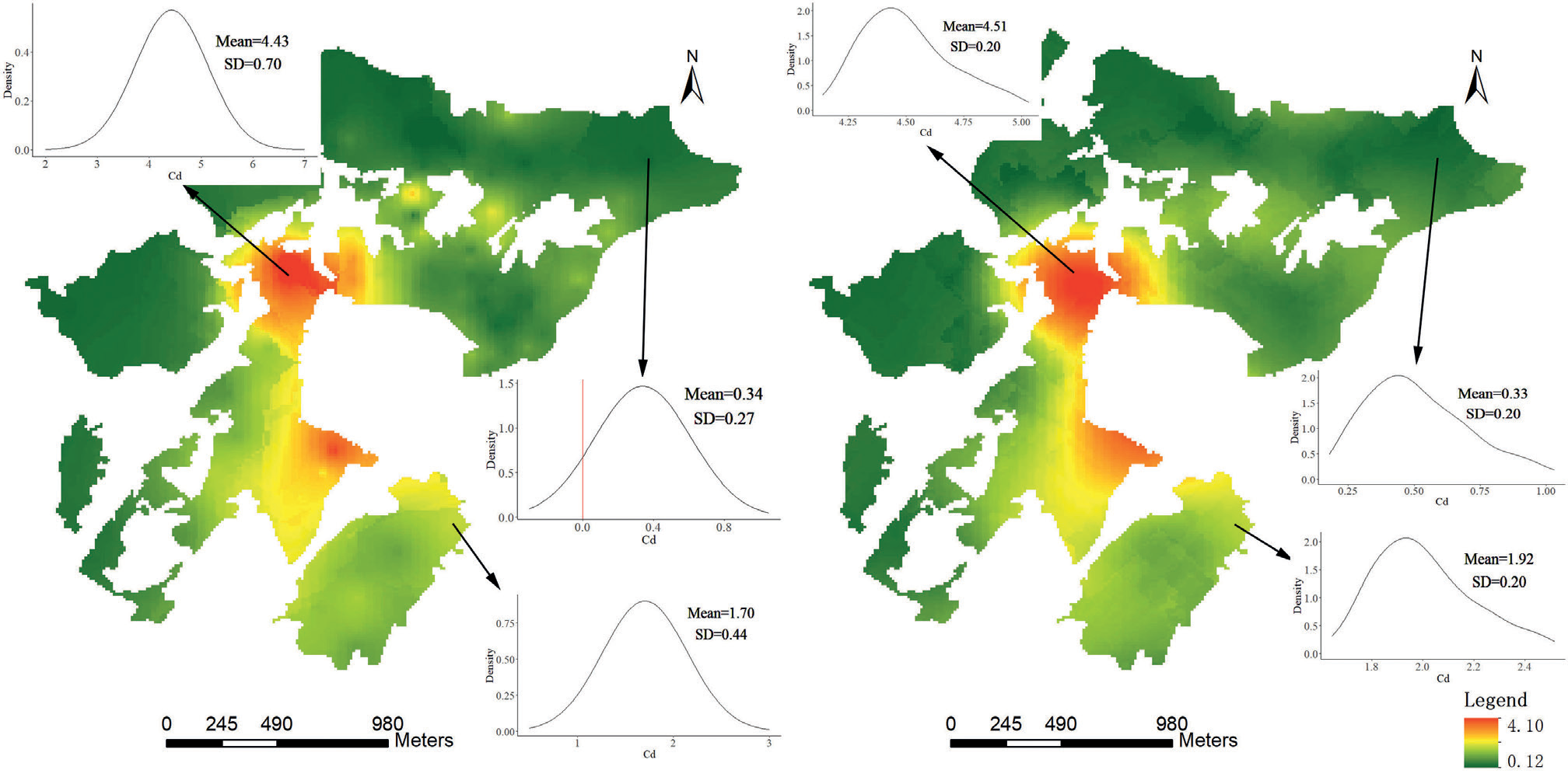
The results of both the copula-based spatial model and the Gaussian spatial model using a Bayesian process have four types of extremal regions, including the Cd concentration of the soil exceeding q.95=2.47 mg/kg with a 50% probability, the Cd concentration of the soil exceeding q.95=2.47 mg/kg with a 75% probability, the Cd concentration of the soil exceeding ConV=3.00 mg/kg with a 50% probability, and the Cd concentration of the soil exceeding ConV=3.00 mg/kg with a 75% probability (Figs. 6 and 7). The red dots in the figures are based on whether the samples exceeded the thresholds. The recognition accuracy was obtained based on whether the red dots were located within the regions above (Table 3). It was found that the recognition accuracies of the copula-based spatial model for regions with Cd concentrations exceeding q.95=2.47 mg/kg with a 50% probability and Cd concentrations exceeding ConV=3.00 mg/kg with a 50% probability were significantly higher than those of the Gaussian spatial model using a Bayesian process. In addition, Fig. 8 shows that the probability density functions (PDFs) of the predicted locations obtained using the copula-based model are closer to the characteristics of the samples, whereas the results of the Bayesian spatial model may produce negative values.
Conclusions
In summary, in this study, the advantages of the copula-based spatial model were demonstrated, and the spatial heterogeneities of the heavy metal concentrations of anthropogenic soil related to mining were determined.
(1) After land consolidation, the heavy metal concentrations of the soil environment in the mining area always exhibit weak random spatial heterogeneity because of soil replacement. Among these heavy metals, several have strong stratified spatial heterogeneity, including Cd and As, in the study area. For this situation, e.g., for Cd and As, the copula-based spatial model may perform better than the spatial model based on the Gaussian assumption.
(2) The spatial heterogeneities of the heavy metal concentrations of anthropologic soil should be explored on two scales, including samples and stratified statistics. The combination of random and stratified spatial heterogeneity can depict the spatial characteristics of anthropological soil well. If some of the factors have strong stratified heterogeneity, the copula-based spatial model may be the better model to use.
Fig. 7.
The areas exceeding the specific thresholds (q.95 and ConV) with a 50% or 75% probability identified by the copula-based spatial model.
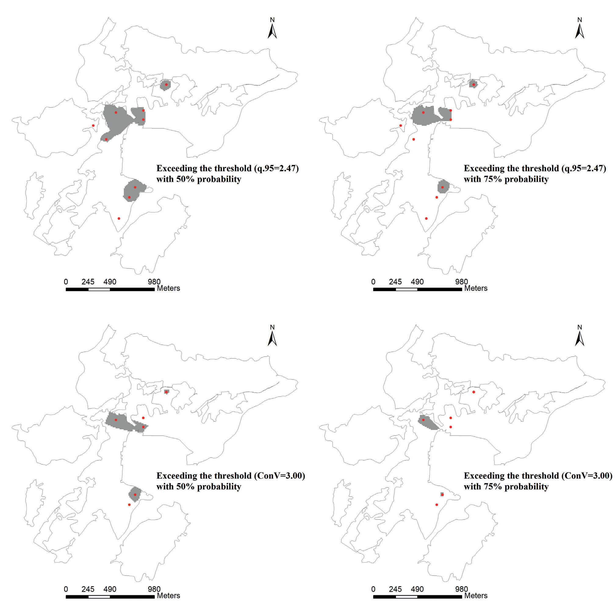
Table 3.
Recognition accuracies of the extremal regions for the different models.
| Gaussian spatial model using a Bayesian process | Copula-based spatial model | |||
|---|---|---|---|---|
| Threshold value | 50% | 75% | 50% | 75% |
| q.95=2.47 | 0.44 | 0.44 | 0.78 | 0.44 |
| Control value=3.00 | 0.33 | 0.33 | 0.67 | 0.33 |
(3) There are many copulas that can be used to fit the spatial rank correlation of the point pairs. The frankCopula, normalCopula, and tCopula have two heavy tails, while the claytonCopula and gumbelCopula have a single heavy tail. These types of copulas can adequately describe the correlation between the marginal distributions because the correlation between the spatial locations depends only on the distance. In addition, the copula-based model always produces better visual results. In the study area, by assessing the copulas for Cd, we determined that the extremal regions appear within a radius of nearly 200 m around the extreme samples with a high probability. In addition, the random error of the variogram fitting was finally summed up as a nugget, but the copula-based spatial model distributes the randomness to every copula in the form of a probability through maximum likelihood estimation. Thus, the predicted results exhibit the characteristics of the raw data rather than a Gaussian distribution.
Fig. 8.
Gaussian spatial distribution of Cd based on a Bayesian process (left) and the copula-based spatial distribution of Cd (right). The predicted PDFs of the three particular points are also shown.
(4) Through identification of the extremal regions of the Cd concentration in the study area, it was determined that the recognition accuracy of the copula-based spatial model was higher than that of the Gaussian spatial model using a Bayesian process. Moreover, the results of the copula-based spatial model are more reasonable (non-negative).

