

Introduction
Over the past century, the rapid development of human society has led to a continuous increase in the consumption of energy sources, such as coal and oil, resulting in a growing volume of greenhouse gas emissions, and an increasingly severe global warming trend. Data released by the International Bank for Reconstruction and Development (IBRD) shows that in 2005, China’s carbon emissions reached a staggering 5.825 billion tons, which made it the world’s leading carbon emitter. Since then, China has topped the list of global carbon emissions. To reduce the emissions, a series of measures have been proposed. The introduction of the Dual Carbon Goals in 2020 further demonstrates China's commitment to a low-carbon development path and its determination to join other countries in addressing the global warming issue.
Located in the North China Plain, the Beijing-Tianjin-Hebei urban agglomeration has a large economic scale and strong development vitality. In 2005, the carbon emissions intensity in the region was 3.50 t CO2/10,000 yuan, but by 2019, it had decreased to 1.49 t CO2/10,000 yuan, marking a reduction of 57.4%. This achieved and exceeded the 2020 carbon reduction target of a 40%-45% reduction in carbon emissions intensity compared to the 2005 level1. However, there is still a long way to go in promoting low-carbon coordinated development in this region. In 2019, the carbon emissions of the Beijing-Tianjin-Hebei urban agglomeration were 1,262.84 million tons, a slight increase compared to 2018. The economic development in this region is not sufficiently balanced, with striking differences in industry and energy consumption structures among cities. Relevant carbon reduction theories, methods, and policy support are in urgent need. In recent years, driven by technologies like artificial intelligence, China is undergoing a transition from traditional economy to digital economy. In 2022, the scale of China’s digital economy reached 50.2 trillion yuan, a 10.3% year-on-year increase2. While the digital economy is rapidly advancing, its ability to improve resource utilization efficiency and drive green technological innovation has led an increasing number of people to study its carbon reduction effects. The overall level of digital economic development in the Beijing-Tianjin-Hebei urban agglomeration ranks at the forefront in China, and significant progress has been made in carbon reduction efforts. Therefore, this region can serve as a good example for research. Exploring driving factors of carbon emissions under the background of digital economy in this region not only provides a theoretical basis for promoting carbon reduction through the regulation of relevant factors, but also serves as a leading and demonstrative role in guiding the formulation of environmental protection measures in other parts of the world, thereby promoting the development of global environmental protection efforts.
Literature Review
Carbon Emission Drivers
The earliest research on factors influencing carbon emissions primarily revolved around three factors: population, affluence, and technology. Many studies indicate that the growth of population and economy plays a promoting role in carbon emissions [1-3]. Zhu and Peng (2012) [4] conducted an in-depth study on the impact of population on carbon emissions and found that changes in population structure, rather than population size, are the main influencing factors on carbon emissions. Regarding the impact of economic growth on carbon emissions, an increasing number of studies have shifted from linear to non-linear models, verifying an inverted U-shaped relationship, where economic growth initially promotes and later inhibits carbon emissions. Bibi et al. (2021) [5] and Aslan et al. (2018) [6] both confirmed this conclusion. As for the impact of technology on carbon emissions, the majority of literature indicates a negative correlation between the two [7, 8]. Chen et al. (2023) [9] decompose technology into production technology, energy-saving technology and energy substitution technology. They found that energy-saving technology and energy substitution technology have a positive reducing effect on carbon emissions, while production technology has almost no impact. In addition to these three factors, a substantial amount of research has found that the increase in the level of urbanization and changes in industrial structure also have a significant impact on urban carbon emissions [10-13].
In the past decade, with the rapid development of digital economy, more and more scholars have begun to explore the impact of digital economic development on carbon emissions. There are currently conflicting opinions on the impact of digital economy on carbon emissions. According to Zhou et al. (2019) [14], the rapid development of the information and communication technology industry has led to an increase in carbon emissions due to the industry’s extensive use of carbon-intensive intermediate products. Dong et al. (2022) [15], using data from 60 countries and regions worldwide, found that the growth of the digital economy has a positive impact on the scale of carbon emissions, but has a negative impact on carbon emissions intensity. Domestic scholars like Xiang et al. (2023) [16], based on panel data of Chinese cities, argue that the development of the digital economy can significantly reduce the carbon emissions intensity in various regions of China. Huo et al. (2022) [17] reached similar conclusions. However, Miao et al. (2022) [18] and Ge et al. (2022) [19] found an inverted U-shaped nonlinear relationship between the development of the digital economy in Chinese cities and carbon emissions.
Research Methods for Analyzing Factors Influencing Carbon Emissions
Currently, there are numerous research methods for analyzing the factors influencing carbon emissions. The mainstream methods include the Logarithmic Mean Divisia Index (LMDI) decomposition method and the extended STIRPAT model analysis method. LMDI decomposition can be traced back to the 1990s [20]. Subsequently, many scholars combined the LMDI decomposition method with the Kaya identity to analyze the factors influencing carbon emissions. O'Mahony (2013) [21] and Mousavi (2017) [22] used the Kaya-LMDI model to decompose the factors influencing carbon emissions in Ireland and Iran, calculating the contributions of various factors to carbon emissions and providing recommendations for carbon reduction. Compared to the LMDI decomposition method, the extended STIRPAT model is more flexible in variable selection and is used by more researchers [23]. When using the linear regression method to analyze the STIRPAT model, serious multicollinearity problems often occur among variables. For this reason, scholars have tried a variety of methods to solve it. These methods can be mainly categorized into three types. The first is traditional subset selection methods, including stepwise regression and optimal subset. Shuai et al. (2018) [24] and Qin et al. (2019) [25] used stepwise regression, sequentially introducing significant variables based on their partial correlation coefficients, to establish a regression equation for investigating the key factors of carbon emissions in China. Tan et al. (2015) [26] established multivariate statistical models through optimal subset regression to predict carbon emissions in Malaysia. Both of these methods address the issue of multicollinearity by adding or removing variables. The second category is shrinkage methods, also known as regularization, which includes ridge regression, Lasso regression, and elastic net. Wang et al. (2013) [27] used ridge regression to fit the extended STIRPAT model to explore the factors influencing carbon emissions in Guangdong Province. This method solved the multicollinearity problem by introducing an L2 regularization term. In addition, many scholars have applied this method to fit models for factors influencing carbon emissions [28-30]. Yang et al. (2018) [31] and Huang et al. (2023) [32] combined the STIRPAT model with principal component analysis and Lasso regression respectively to explore the influencing factors of carbon emissions. Different from ridge regression, Lasso regression solves the multicollinearity problem by introducing the L1 regularization term. The third category is dimensionality reduction methods, including principal component regression(PCR) and partial least squares regression(PLSR). Zhang et al. (2014) [33] used PCR to eliminate multicollinearity among various influencing factors of carbon emissions. Since PCR only considers the explanation of independent variables, PLSR also considers whether the extracted principal components have the greatest explanatory power for the dependent variable. Therefore, PLSR is considered to be better than PCR. Li et al. (2020) [34] and Su et al. (2020) [35] used the PLSR method to analyze the influencing factors of carbon emissions in Shanghai and Fujian Province, China respectively.
In addition to the LMDI decomposition method and the extended STIRPAT modeling approach, some other methods have also been used for the research of factors influencing carbon emissions. For instance, Wang et al. (2021) [36] used the random forest method in machine learning to analyze the influencing factors of carbon emissions in 73 cities along the Yangtze River Economic Belt, and conducted an analysis based on regional differences. Yu et al. (2022) [37] used a Panel Vector Autoregression (PVAR) model to examine the long-term dynamic relationships between carbon emissions, imports of cultural products, income, and other variables.
Research on Carbon Emissions in the Beijing-Tianjin-Hebei Region
The relevant research on carbon emissions in the Beijing-Tianjin-Hebei region has been concentrated on the period after 2015. Wen et al. (2016) [38] set up different development scenarios to predict the carbon emission peak before 2050 in the Beijing-Tianjin-Hebei region, and put forward a series of carbon emission reduction suggestions. Research by Bai et al. (2021) [39] found that Hebei’s carbon emission reduction process is slower than that of Beijing and Tianjin, which is more obvious in less developed cities in Hebei. Zhang et al. (2019) [40] pointed out that, compared to Beijing and Tianjin, Hebei has greater potential in carbon emissions reduction and should take on more responsibilities. Wang et al. (2022) [41] and Li et al. (2023) [42] respectively studied the factors influencing carbon emissions in the Beijing-Tianjin-Hebei region from the perspectives of supply-side reform and the industrial chain.
A comprehensive review of existing research reveals the following main shortcomings:
(1) Analyses of the factors influencing carbon emissions in the Beijing-Tianjin-Hebei region mostly remain at the provincial level, with relatively few studies exploring the topic at the city level. Research conducted at the city level can better capture regional variations and provide a larger sample size.
(2) When applying the extended STIRPAT model to analyze factors influencing carbon emissions, most literature tends to use ridge regression methods to address multicollinearity issues, with minimal utilization of partial least squares regression. However, in cases where there are numerous independent variables and a limited sample size, PLSR can better handle high-dimensional data through dimensionality reduction, thereby achieving estimates superior to ridge regression.
(3) When investigating the impact of digital economy on carbon emissions, most literature conducts overall analyses of the study area without considering variations in the digital economic development within regions.
To address the aforementioned issues, this paper takes the data of 13 cities in the Beijing-Tianjin-Hebei region from 2011 to 2019 as samples, then uses the entropy method to calculate the development level of the digital economy and extends it to the STIRPAT model. Finally, the impact of each factor on carbon emissions is evaluated through the PLSR method. Moreover, considering the significant regional differences in the level of digital economic development in the Beijing-Tianjin-Hebei region, hierarchical clustering is used to classify cities into three categories for comparative analysis and presents tailored proposals. On the one hand, this paper aims to investigate whether and how digital economy affects carbon emissions, while also discussing the impact of other factors on carbon emissions. On the other hand, using the Beijing-Tianjin-Hebei urban agglomeration in China as a research sample, it can provide reference and inspiration for carbon reduction in other regions worldwide. Therefore, the paper holds significant theoretical and practical guidance implications.
Material and Methods
STIRPAT Model
In 1997, Dietz and Rosa proposed a stochastic model capable of hypothesis testing, the Stochastic Impacts by Regression on Population, Affluence, and Technology (STIRPAT) model, to explain the impact of human activities on the environment [43]:
where I, P, A, and T represent the environmental impact, population size, affluence, and technological level, respectively. In this paper, I is characterized by carbon emissions and denoted as C. P, A, and T are year-end population (in millions), per capita GDP (in ten thousand yuan per person), and energy intensity (in tons of standard coal per hundred thousand yuan), respectively. To investigate the impact of digital economic development on carbon emissions, the level of digital economic development (D) is introduced into the model. Furthermore, two additional variables, urbanization rate (U) and industrial structure (the proportion of the secondary industry in GDP, S), are included in the model. Finally, the extended STIRPAT model is obtained as Equation (1).
To address heteroscedasticity in the data, taking the logarithm of both sides of Equation (1) yields Equation (2), where the independent variables are lnD, lnP, lnA, lnT, lnU and lnS, the dependent variable is lnC, lna is the constant term, lne represents the error term, and β1~β6 are the elasticity coefficients for each independent variable.
PLSR Algorithm
When using the ordinary least squares method for regression analysis, if there is a multicollinearity problem between variables, the estimated coefficients and significance will be invalid [44]. PLSR is a regression method suitable for small sample sizes and able to address multicollinearity problems without the need to remove any independent variables. It was first proposed by Wold and Albano. The specific modeling steps for the single-factor PLSR model are as follows3 [45].
Principal Component Extraction
After standardizing the dependent variable y(y∈Rn) and the set of independent variables X(X = (x1, x2, ···, x6), xj∈Rn) separately, we can obtain Y0(Y0∈Rn) and X0. By extracting one component t1 from X0 , t1 = X0w1, ||w1|| = 1, we can calculate w1 :
By implementing regression of X0and Y0 on t1, X0 = t1p1T + X1 and Y0 = t1r1+Y1, where p1 and r1 are regression coefficients. The corresponding residual matrices are X1 = X0-t1p1T and Y1 = Y0-t1r1. Then, X0 is replaced by X1 and Y0 by Y1 , the above operations are repeated to obtain w2, t2, X2, Y2, ... , and the iteration is continued accordingly. Cross validity can be used to determine the number of extracted components th to stop the iteration.
Calculating the Regression Model
After obtaining the component t1,t2, ···, tm(m<A, A = rank(X)), the regression model of Y0 with respect to t1,t2, ···, tm is as follows:
where
By following the standardized reverse process, Equation (5) can be converted back into its non-standardized form.
Analysis of Carbon Emissions in the Beijing-Tianjin-Hebei Urban Agglomeration
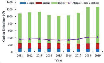
The carbon emissions data in this paper are obtained from the China Emission Accounts and Datasets (CEADs)4. This dataset takes into account carbon emissions from 47 social and economic sectors, 17 types of fossil fuels, and cement production processes, with comprehensive and reliable results [46-49]. The carbon emissions data from 11 prefecture-level cities in Hebei Province are aggregated at the provincial level and plotted in Fig. 1. From the figure, it can be observed that, between 2011 and 2019, the total carbon emissions in the Beijing-Tianjin-Hebei region showed a decreasing trend from 2013 to 2015 and an increasing trend in other years. Hebei had the highest carbon emissions, followed by Tianjin, and Beijing had the lowest. Lower carbon emissions in Tianjin and Beijing indicates that Hebei was the dominant source in this region.
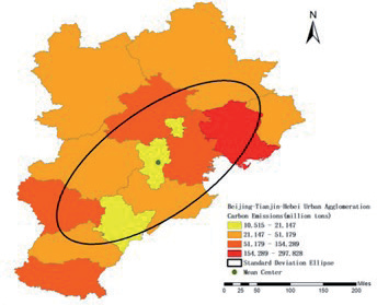
To further explore the spatiotemporal variations in carbon emissions among the 13 cities, ArcGIS 10.7 software is utilized to create carbon emissions distribution maps for the Beijing-Tianjin-Hebei urban agglomeration in 2011 and 2019. Additionally, tools such as the mean center and standard deviation ellipse are used to compare the spatial distribution differences in carbon emissions between different periods. The changes in the carbon center of the region from 2011 to 2019 are illustrated in Fig. 2 and Fig. 3, and relevant geographic parameters are provided in Table 1.
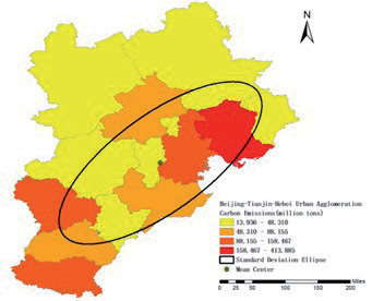
Table 1.
Carbon center parameters.
| Year | Longitude | Latitude | Location |
|---|---|---|---|
| 2011 | E 116°37'22.637'' | N 39°4'38.506'' | Langfang City, Bazhou District |
| 2019 | E 116°46'5.862'' | N 39°2'30.537'' | Tianjin City, Jinghai District |
From Fig. 2 and Fig. 3, it can be observed that the major axis of the carbon emissions standard deviation ellipse in the Beijing-Tianjin-Hebei region is oriented in the southwest-northeast direction. Moreover, the ratio of the ellipse’s major axis to its minor axis is relatively large, indicating that the distribution of carbon emissions in this region is not uniform, and there is a significant spatial variation in carbon emissions among the cities [50]. Carbon emissions in the Beijing-Tianjin-Hebei region are primarily concentrated around the Beijing-Tianjin-Tangshan and Shijiazhuang-Handan areas. From 2011 to 2019, there was an eastward shift in the carbon center of this region, transitioning from Bazhou District in Langfang City to Jinghai District in Tianjin City, with an increasingly pronounced spatial disparity in carbon emissions.
Measurement and Regional Classification of Digital Economic Development Level
Indicator Selection
Based on the review of literature, this paper constructs a measurement system for the development level of the digital economy from four dimensions: digital infrastructure, digital industry development, digital innovation capability, and digital inclusive finance [51, 52] (Table 2). Using this system, the digital economic development index for 13 cities in the Beijing-Tianjin-Hebei region from 2011 to 2019 is calculated. Data for each indicator are obtained from “China City Statistical Yearbook,” “Hebei Statistical Yearbook,” the State Intellectual Property Office, and the Peking University Digital Inclusive Finance Index. A small amount of missing data can be supplemented through linear interpolation and exponential smoothing methods.
Calculation of Digital Economic Development Index
The entropy method is used to assess the level of digital economic development. According to the method used by the World Economic Forum to construct the Network Readiness Index (NRI) [53], all indicator data in the paper are standardized and controlled within the range of 1-7. By calculating the information redundancy, the weights of each indicator are obtained. Based on the weighted indicators, a linear weighted calculation is performed on the standardized data to obtain the Digital Economic Development Index of 13 cities in the Beijing-Tianjin-Hebei region for the years 2011-2019 (Table 3).
From Table 3, it can be seen that the digital economic development in the Beijing-Tianjin-Hebei region showed an overall upward trend between 2011 and 2019. Among the 13 cities, Beijing had the highest level of digital economic development, far surpassing the other 12 cities, with Tianjin ranking second. In Hebei Province, the 11 prefecture-level cities were ranked from 3rd to 13th, with Shijiazhuang, Langfang, and Qinhuangdao taking relatively higher levels, while Handan, Xingtai, and other areas had lower levels. In terms of growth rate, Zhangjiakou, Baoding, and Xingtai had a relatively high increase in their digital economic development in 2019 compared to 2011, all exceeding 90%, while Tianjin, Tangshan, and Handan had lower growth rates, all below 80%.
Table 2.
Indicator system for the level of development of the digital economy.
Table 3.
Beijing-Tianjin-Hebei Urban Agglomeration Digital Economic Development Index.
Hierarchical Clustering
Considering the significant regional disparities in the level of digital economic development within the Beijing-Tianjin-Hebei urban agglomeration, and the varying impact of different levels of digital economic development on carbon emissions, this paper categorizes the 13 cities in the Beijing-Tianjin-Hebei region into three groups based on their levels of digital economic development for separate analysis. In contrast to the subjective division into high, medium, and low categories of the Digital Economic Development Index, the use of hierarchical clustering is more objective and reasonable. As an unsupervised learning approach, hierarchical clustering continuously merges similar samples into clusters by calculating the distances between samples. Eventually, all samples are merged into one large cluster. In this paper, the 2019 Digital Economic Development Index of the 13 cities is taken as the samples, and the Ward method (sum of deviation square method) is used for hierarchical clustering. When class Gp and class Gq are merged into class Gr , the formula for calculating the distance between class Gr and other class Gk is shown as Equation (6), where ni is the number of samples included in class Gi, and the inter-class distance D is calculated from the sum of squared deviations. The hierarchical clustering dendrogram (Fig. 4) is generated based on the calculation results [54].
Fig. 4.
Hierarchical Clustering Dendrogram. Note: In the picture, BJ, TJ, SJZ, QHD, LF, TS, BD, HD, XT, CZ, HS, ZJK, and CD respectively represent Beijing, Tianjin, Shijiazhuang, Qinhuangdao, Langfang, Baoding, Hengshui, Xingtai, Cangzhou, Hengshui, Zhangjiakou, and Chengde.
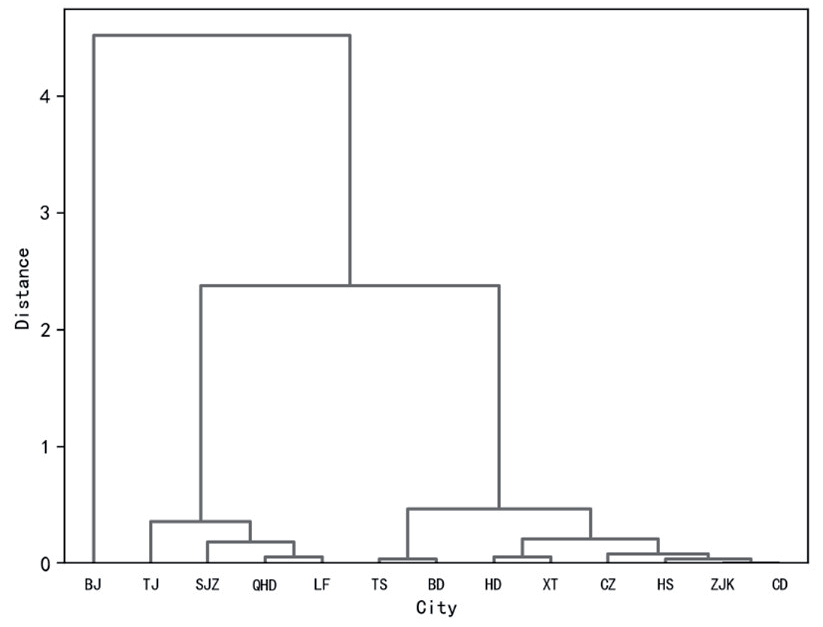
As shown in Fig. 4, Beijing has the highest level of digital economic development, forming a separate category labeled as H region. Tianjin, Shijiazhuang, Qinhuangdao, and Langfang are intermediate, forming the M region. The remaining eight cities, including Tangshan and Baoding, exhibit relatively lower levels of digital economic development and are designated as the L region. The specific classification details are presented in Table 4.
Results and Discussion
Descriptive Statistics
This study is based on Equation (2), in which carbon emissions and the digital economic development index have been explained above, and the remaining variables are taken from “China Statistical Yearbook” and “China Urban Statistical Yearbook.” The descriptive statistics for each variable are presented in Tables 5-7.
Multicollinearity Test
H region (Beijing) is adopted as an example and a correlation test is conducted on each independent variable. The results are shown in Table 8. It can be observed that the independent variables are not mutually independent, indicating a severe multicollinearity problem. By calculating the Variance Inflation Factor (VIF) values of the influencing factors through Ordinary Least Squares (OLS) regression (Table 9), for all six factors the VIF values far exceed the upper limit of 10. This suggests that the coefficients and their significance obtained from the OLS regression are not reasonable and cannot serve as the basis for analysis.
Table 4.
Regional Classification of Digital Economic Development Levels in the Beijing Tianjin-Hebei Urban Agglomeration.
Table 5.
Descriptive statistics of variables in the H Region from 2011 to 2019.
Table 6.
Descriptive statistics of variables in the M Region from 2011 to 2019.
Table 7.
Descriptive statistics of variables in the L Region from 2011 to 2019.
Partial Least Squares Regression (PLSR)
To address the problem of multicollinearity, this study employs PLSR to analyze the log-transformed extended STIRPAT model (Equation 2).
Table 8.
Correlation Test Results.
Table 9.
Multicollinearity Test Results.
| Variable | VIF | 1/VIF |
|---|---|---|
| lnD | 1422.99 | 0.000703 |
| lnU | 1347.29 | 0.000742 |
| lnP | 1307.52 | 0.000765 |
| lnS | 761.37 | 0.001313 |
| lnA | 248.41 | 0.004026 |
| lnT | 65.82 | 0.015194 |
| Mean VIF | 858.9 |
Determination of Model Principal Components
All analyses related to PLSR in this study are carried out using SIMCA 14.1 software. Initially, the number of model principal components is determined through a cross-validity test, and the cross-validity indicators are presented in Table 10. In the table, R2X(cum) and R2Y(cum) respectively represent the percentage of X and Y matrix information that the PLSR model can explain, and Q2(cum) is used to evaluate the predictive ability of the model. When Q2≥0.0975, adding new principal components significantly improves the model; otherwise, the further introduction is halted [55]. Based on the cross-validity indicators, 1, 4, and 5 principal components were successively extracted for the three regions. It can be observed that R2X(cum), R2Y(cum), and Q2(cum) all exceed 0.7, indicating that the established PLSR model is relatively precise, and the number of extracted principal components is reasonable.
Identification of Specific Points
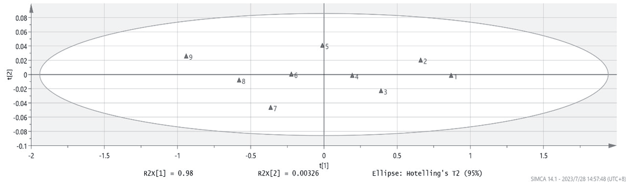
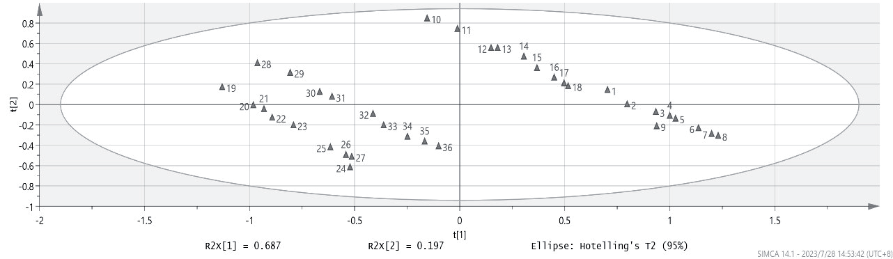
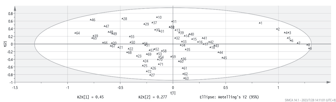
In PLSR, the presence of specific points can affect the model’s fitting performance, and they need to be removed before refitting the model. The T2 elliptical figure is used to observe the distribution and similarity structure of sample points on the T1/T2 plane, and it can identify specific points with values far from the average level of the sample point set [56]. As seen from Fig. 5, Fig. 6, and Fig. 7, the sample points from the three regions all fall within the T2 ellipse. Therefore, there are no specific points, and subsequent analysis can be carried out.
Table 10.
PLSR cross-validity indicators.
Regression Results and Variable Importance in Projection (VIP)
For each of the three regions, a PLSR model is constructed with the appropriate number of principal components. The standardized coefficients for each variable are shown in Table 11. These standardized coefficients are then transformed into their non-standardized form, yielding non-standardized estimation equations for the three regions:
H region:
M region:
L region:
In PLSR, the commonly used indicator for comparing the explanatory power of various independent variables on the dependent variable is called Variable Importance in Projection (VIP). The calculation method for this indicator is shown in Equation (7) [45], where whj is used to measure the marginal contribution of the independent variable xj to the construction of component th, and Rd(Y;t1, ···, tm)represents the cumulative explanatory power of components t1, ···, tm on the dependent variable, carbon emissions. For H, M, and L regions, m is 1, 4, and 5 respectively.
When VIP≥1, it is considered that the variable has a significant impact on carbon emissions. When 1>VIP≥0.5, the impact is moderate. When 0.5>VIP≥0.2, the impact is relatively small. However, when VIP<0.2, it is considered that the variable has almost no impact on carbon emissions.
Empirical Results Analysis
As shown in the results of Table 11, The VIP values of almost all variables are greater than 0.2, which supports the rationality of the selection of influencing factors and the setting of the extended STIRPAT model. On the whole, the results show that, like the traditional factors of population, affluence and technology, the digital economy and industrial structure have also proved to produce a non-negligible impact on the carbon emissions of the Beijing-Tianjin-Hebei urban agglomeration. More importantly, the impact of these factors on carbon emissions shows a general and significant difference in the three regions. In this regard, we will analyze one by one according to the influencing factors:
(1) Digital economy. The results in Table 11 reveal that the estimated coefficients of lnD are all negative under the H, M and L regions, and the VIP values are all greater than 0.5, indicating that the digital economy has a stable and significant inhibiting effect on carbon emissions. This is consistent with the finding of Zhu et al. [52]. The digital economy mainly affects carbon emissions from two aspects of enterprise production and governance. On the one hand, by utilizing more data and information, digital technology can directly optimize a company’s production solutions, which reduces energy waste and contributes to carbon reduction, such as the use of unmanned workshops and smart logistics. On the other hand, digital technology facilitates the sharing of knowledge elements and the allocation of market resources, which promotes green technological innovation and the development of the carbon trading market, thereby improving the governance of carbon emissions. What’s more, from the value of the estimated coefficient (L: -2.4536<M: -0.8288<H: -0.0974), we can further find that the carbon emission reduction effect of the digital economy is characterized by marginal decline. This implies a late-mover advantage, that is, cities at a lower level of digital economic development will have a stronger potential to reduce carbon emissions, which does not support the more common U-shaped conclusion [18, 57, 58]. A reason for this may be that the development of the digital economy in the Beijing-Tianjin-Hebei region was already at a high level during the observation period, and the relationship between the digital economy and carbon emissions had already passed the inflection point period.
(2) Population. There is a clear regional heterogeneity in the impact of population on carbon emissions, but with little difference between the effects of population size (total population) and population structure (urbanization rate). As can be seen from Table 11, the estimated coefficients of lnP and lnU are both negative and the VIP values are less than 0.5 in region H. In regions M and L, the estimated coefficients of lnP and lnU are both positive and the VIP values are greater than 0.5. All results suggest that demographic factors, both in terms of size and structure, remain important factors in the growth of carbon emissions in regions M and L, but not in region H. This is in line with the actual situation of population growth in the Beijing-Tianjin-Hebei region. In region H, i.e. Beijing, the total population has not grown since 2016 and the urbanization rate has remained above 85%. Its demographic situation has basically stabilized, so the impact of population on carbon emissions is weak. In contrast, population changes are more pronounced in Hebei and Tianjin, especially the urban population. From 2011 to 2019, the urban population of Hebei has increased by 13.22 million, and the urbanization rate increased by 16 percentage points. Tianjin’s total population has risen by 18% and the urbanization rate has increased by nearly 10 percentage points. The massive influx of people from rural to urban areas has created more demand for energy from both living and production sources, which has led to an increase in carbon emissions in these regions [4].
(3) Regional affluence. As for GDP per capita, its estimated coefficient is still significantly positive in region L, but the opposite result is obtained in other regions, which demonstrates that the positive correlation between urban economic growth and carbon emissions will be eroded in regions with high levels of digital economic development. This is because the development of digital economy has also led to the development of low-carbon economy to a certain extent, which reduces the dependence on energy. As the core industry of the digital economy, the ICT industry has inherent low-carbon attributes. The technical characteristics of “virtual” and “dematerialization” make its economic activities not directly dependent on fossil energy [59]. Moreover, the combination of digital technology and traditional industries has also led to the transformation and upgrading of industrial structure, which has improved production efficiency and promoted the development of an intensive economy [52]. More generally, H and M regions also have higher per capita GDP. As shown in Tables 5 to 7, the average per capita GDP of H and M regions in 2011-2019 is 113,400 and 63,500 yuan, respectively, which is 2.94 and 1.65 times that of L region. According to the environmental Kuznets curve theory, the economic growth of these regions with higher GDP per capita no longer increases carbon emissions, but rather has a dampening effect.
Table 11.
PLSR coefficients of influencing factors.
(4) Technology level. As shown in Table 11, the estimated coefficients of lnT in the H, M, and L regions are 0.1133, -1.1237, and-1.4059, respectively, and the VIP values are all greater than 1.0. The results show that technological progress will be conducive to the reduction of carbon emissions in H area, but not conducive to M and L areas. In other words, the energy rebound effect is proved to exist, but only in M and L regions. This is closely related to the industrial structure in three regions. The results in Tables 5 to 7 show that the share of the secondary sector in Region H is only 20.25%, which is much lower than 42.88 % and 47.66 % in the M and L regions. Manufacturing still occupies a high proportion in M and L regions, and the consumer demand for industrial products is still strong in both regions. Therefore, the decline in energy costs brought about by technological progress has not only failed to reduce total energy consumption, but has stimulated consumption demand and ultimately led to an increase in carbon emissions [60]. In Beijing (Region H), where the focus of economic development has long since shifted to greener service industry, advances in energy-saving technologies may further deepen the concept of low-carbon consumption, so the effect of energy conservation and emission reduction will be more pronounced. However, how the industrial structure affects the carbon emissions in these areas, we will discuss in the next paragraph.
(5) Industrial structure. The estimation coefficient of lnS is significantly positive in H region and negative in another two regions, indicating that the proportion of secondary industry in Beijing has a positive relationship with carbon emissions, and has a reverse relationship in M and L regions. Since the proportion of the secondary industry in Beijing, Tianjin and Hebei actually showed a downward trend (i.e., industrial structure upgrading) during the sample observation period, the results further revealed that the upgrading of industrial structure could not effectively reduce the total carbon emissions in Hebei and Tianjin, which was contrary to the research conclusions of Yang et al. and Wu et al. [61, 62]. However, combined with the actual industrial development in the Beijing-Tianjin-Hebei region, we can pry into some reasonable explanations. Firstly, manufacturing remains an important pillar of economic growth in Tianjin and Hebei, with an average contribution rate of 37% and 38.1%, respectively, much higher than Beijing’s 18%. Although the proportion of manufacturing industry in Hebei and Tianjin is declining, the scale has increased by 62.5% and 50.7% respectively, which greatly weakens the carbon reduction effect of industrial structure upgrading. Secondly, as the largest carbon emission sector [63], there are significant differences in the development of the construction industry in the three regions. Compared with Beijing and Tianjin, the proportion of the construction industry in Hebei has increased instead of decreasing (from 5.6% to 5.9%), which has promoted the growth of major carbon emissions in M and L regions.
Conclusions and Policy Recommendations
Nowadays, with the continuous breakthrough of digital core technology represented by artificial intelligence, the development of digital economy has brought earth-shaking changes to residential life and enterprise production. So, as a hot topic in China’s urban economy, how does it affect carbon emissions? Driven by digital technology, how has the relationship between traditional factors and carbon emissions changed? To answer these questions, based on the panel data of Beijing-Tianjin-Hebei urban agglomeration in China from 2011 to 2019, this paper uses STIRPAT model and PLSR method to systematically explore the influencing factors of carbon emissions in Beijing-Tianjin-Hebei region after considering the factors of digital economy. In order to better observe the regional heterogeneity characteristics of their influences, we divided all cities into three categories according to the level of digital economic development, namely H, M and L regions, and conducted a sub-sample regression.
Our research mainly draws the following conclusions: (1) Compared with the performance of other factors in different regions, the digital economy is the most stable source of carbon reduction, which has a significant inhibitory effect on carbon emissions in all regions. However, the carbon reduction capacity of the digital economy will decline as the level of digital economy development continues to rise. (2) Traditional demographic, economic and technological factors still limit low-carbon development in M and L regions, which has a strong positive correlation with carbon emissions. Nonetheless, this relationship does not exist in H-Region. (3) The carbon-reducing effect of industrial structural upgrading has proven to be a failure. In M and L regions, the decline in the share of secondary industry plays a positive role on carbon emissions.
There are also many studies on the influencing factors of carbon emissions and the impact of digital economy on carbon emissions [4, 7, 12, 18, 19, 52]. The difference with these studies is that we use a new methodology and a new sample. The introduction of the PLSR method solves the multicollinearity problem that traditional OLS estimation is difficult to overcome, which makes our research conclusions more convincing than other studies. Taking the Beijing-Tianjin-Hebei urban agglomeration as a sample, rather than all provinces or cities, we also provide a new and more specific evidence for the carbon reduction effect of the digital economy. All the findings expand the application scope of STIRPAT theoretical model, as well as enriching the related research on digital economy and carbon emissions. In addition to the academic value, some important implications are also proposed.
(1) Accelerate the process of urban digitization and build a new pattern of digital economy. At present, the difference in digital economy development within the Beijing-Tianjin-Hebei city cluster is too large, which is not conducive to the improvement of the overall digital economy level in the region. In this regard, the radiation effect of Beijing’s digital economy should be enhanced, while accelerating the pace of digital economy development in other regions. In terms of overall layout, more efforts should be made to support Tianjin to rapidly become the second growth pole of digital economy development in the city cluster, so as to form the “2+11” pattern of coordinated development of digital cities. From the perspective of policy practice in each region, Beijing should accelerate the construction of “digital economy benchmark city”, especially digital core technology innovation, such as precision sensors, integrated circuits, operating systems, industrial software, and databases, etc., so as to provide technological support for the development of digital industries in other regions. Tianjin should constantly enrich digital application scenarios and improve the digital industrial chain, and strengthen technical exchanges and cooperation with Beijing. Hebei should continue to increase the construction of digital infrastructure, such as cross-regional data centers and cloud computing platforms, and quickly expand the overall scale of digital economy.
(2) Improve the quality of urbanization and advocate a low-carbon lifestyle. For M and L regions, the rise of urbanization level and the expansion of population size are the two major obstacles to carbon emission reduction. It does not work to simply reduce the population or lower the urbanization rate. Instead, the following two aspects can be considered: Firstly, considering that cities in Hebei are experiencing a rapid increase in urbanization rates, construction experiences of Beijing and Tianjin should be followed. Urban planning and land-use management should be strengthened to avoid disordered construction and excessive development. Furthermore, low-carbon lifestyles should be actively promoted among the public, such as walking, cycling, and energy conservation, to reduce the negative environmental impact of individual lifestyles.
(3) Deepen industrial transformation and optimize energy structure. In recent years, cities in the Beijing-Tianjin-Hebei region have been undergoing industrial transformation and upgrading, as well as improvement of energy utilization technologies, which have yielded positive carbon reduction results. Currently, energy intensity and the proportion of the secondary industry in Beijing have decreased to relatively low levels, leaving limited room for further carbon reduction. In contrast, other areas in the Beijing-Tianjin-Hebei region, especially heavy industrial cities like Tianjin and Tangshan, still need to promote carbon reduction by optimizing their industrial structure and improving energy efficiency. First of all, Tianjin and Hebei should strengthen cooperation with Beijing in high-tech industries, actively foster emerging industries, and promote industrial transformation and upgrading. Secondly, as China’s major steel production province, Hebei needs to control high carbon-emitting industries and curb the expansion of heavily polluting industries. In addition, for areas with intensive secondary industries in the urban agglomeration, there should be active promotion of clean energy adoption, along with research and application of energy-saving technologies to enhance the energy efficiency of relevant facilities.
However, this paper still has some limitations. First, since the PLSR approach does not overcome the endogeneity problem, the relationship between digital economy and carbon emission obtained in this paper is a correlation relationship rather than a causal relationship, which may reduce the persuasiveness of the explanation and the reliability of the recommendations. Correspondingly, as the PLSR method cannot identify a causal relationship, we have not been able to dig deeper into the impact mechanism of the digital economy on carbon emissions, but only explored the heterogeneous effects of its region. The solution of these problems needs the improvement of PLSR tools and further research in the future.