

Introduction
In response to global climate change, China has committed to peaking carbon emissions by 2030 and achieving carbon neutrality by 2060. The report from the 20th Party Congress emphasized green transformation as a key component of Chinese modernization and ecological progress. In this transformation, GF plays a crucial role in enabling sustainable development, environmental protection, and a low-carbon economy through policies and measures implemented by the government and financial regulators. Innovations in credit, insurance, industrial funds, and institutional arrangements guide investment toward low-carbon, clean energy projects, prompting a shift in funds from high-pollution to low-pollution and ecological protection sectors.
In this context, ANPSP – one of the most challenging environmental issues for developing countries – poses a significant threat to sustainable development [1]. Due to the prolonged use of chemical fertilizers, nitrogen, and phosphorus surpluses during the cultivation of 54 crops in China currently reach 138-421 kg/hm² and 19-118 kg/hm², respectively. The effective phosphorus content of the soil has increased approximately 2.34 times since 1980 [2], while COD, TN, and TP levels associated with ANPSP in China have risen by 91.0%, 196.2%, and 244.1% from 1978 to 2017. Although China has only 7% of the world’s arable land, it consumes one-third of the global fertilizer volume, with application rates 2.6 times the global average. China’s ANPSP has exhibited a pattern of fluctuation, including periods of linear growth [3]. Since the reform era, TN and TP nutrient loading in major lakes and water systems has intensified, with research indicating that agricultural surface and rural pollution predominantly affect water quality. In Europe, agriculture accounts for roughly 33% of water use and is the primary source of nutrient discharge into water resources (EEA Report No. 1/2012) [4].
Globally, sustainable development has gained attention, as exemplified by the UN’s Sustainable Development Goals (SDGs) and the Paris Agreement, which provide frameworks for achieving sustainability. The pursuit of sustainable development spans multiple disciplines, emphasizing effective financial flows, scientific regulation, and efficient resource allocation. Studies, such as those by IŞık et al., reveal that environmental factors play a crucial role in the SDGs, particularly for China [5]. In developing countries, balanced economic growth and environmental protection are essential, as environmental degradation hinders stable growth [6]. Finance has emerged as a critical enabler for environmental sustainability, with many studies highlighting the positive influence of GF on carbon-intensive and energy-based industries [7]. However, while GF’s environmental benefits are well-documented – especially regarding carbon emissions and energy sectors – few studies explore its relationship with ANPSP [8, 9].
GF is central to China’s “14th Five-Year Plan” for green development, offering potential benefits to ANPSP management yet facing obstacles such as uneven financial development. This paper addresses the following questions: What impact does GF have on ANPSP management in China? Does it effectively support ANPSP management? What mechanisms facilitate GF’s role in ANPSP management? This study offers three main contributions: First, it examines the pollution mitigation effect of GF from an agricultural perspective, emphasizing GF’s importance and application in agriculture. Second, it empirically investigates how GF reduces ANPSP through ER and LAND, providing evidence for enhancing China’s GF system. Third, it explores the heterogeneity between GF development and ANPSP across economic levels, offering policy guidance for ecological advancement in China and insights for other developing nations managing surface pollution.
Literature Review
GF originated from the Paris Agreement under the United Nations Framework Convention on Climate Change (UNFCCC), addressing not only traditional environmental concerns but also the challenges associated with financing environmental transformation. The Sustainable Development Goals (SDGs), proposed by the United Nations in 2015, are central to this initiative. IŞıK et al. empirically examined the impacts of the SDGs on the U.S. by selecting 17 representative variables [10]. SDGs have been widely studied across various fields due to their integrated approach, with carbon emissions – a crucial aspect of environmental protection – prominently featured in sustainable development. IŞıK et al. found that re-export shares show a significant relationship with greenhouse gases [11]. ESG (Environmental, Social, and Governance) factors are closely related to firm-level dynamics; however, very few studies incorporate economic factors into sustainability assessments. By adding economic factors (ECON) to the traditional ESG framework, IŞıK et al. developed an econ-ESG model and investigated its relationship with natural resource rent (NR) dynamics [12]. In G7 countries, economic factors negatively impact energy efficiency, while environmental factors exhibit a positive influence [13]. This suggests that economic growth is essential for achieving the SDGs, while the environmental dimension largely depends on financial system development.
Numerous scholars have explored ways to reduce greenhouse gas emissions to achieve the SDGs, considering various strategies such as information communication technology and renewable energy initiatives [14]. Recently, GF has gained substantial attention in academic discourse. As an economic activity supporting environmental improvement, climate change response, and efficient resource utilization, GF has been widely adopted internationally. In order to achieve environmental protection and economic growth, developed countries have implemented a range of financial instruments, including green industry funds, green securities funds, green development banks, and green financial bonds [15]. To foster ecological civilization, China has vigorously promoted GF. The Guiding Opinions on Building a Green Financial System emphasize that GF should not only improve environmental quality and mitigate climate change but also address resource scarcity by channeling investments into environmental protection, energy efficiency, and clean sectors. According to Wind data, China issued 802 green bonds totaling 1,118.05 billion yuan in 2023, marking two consecutive years with issuance volumes surpassing one billion yuan. This underscores China’s commitment to pollution prevention and emission reduction in its new phase of development.
Currently, many scholars focus on the effects of GF development on climate [16]. However, the global issue of agricultural pollution cannot be overlooked. In this new phase of development, China has introduced a series of financial measures that have attracted international attention. While recent years have seen significant progress in addressing agricultural pollution, challenges remain. Integrating market-oriented economic mechanisms with a government-led system to reduce agricultural pollution is crucial. As a market-driven tool, GF has garnered attention regarding its potential to play an even greater role. From a financial perspective, the introduction of GF is conducive to improving agricultural total factor productivity, enhancing resource allocation efficiency, and thus reducing carbon emissions [17]. It also promotes micro-enterprise development, supports agricultural industry modernization, and contributes to cleaner production [18]. Encouraging green innovation [19], LAND [20], financial support, and expanded operational scale can further stimulate agricultural development [21]. From an ANPSP reduction perspective, the over-application of chemical fertilizers and residential activities are primary contributors. Studies measuring green development levels in major food-producing areas from 2011 to 2019 concluded that financial inclusion can mitigate agricultural pollution [22]. Additionally, some scholars [23] argue that reducing farm numbers could help control ANPSP in China. Despite GF’s significant role in reducing carbon emissions, its impact on agricultural pollution remains less clear.
Current research on the management of agricultural land-based pollution primarily emphasizes government-led administrative approaches, while studies exploring GF as a tool for managing land-based pollution remain limited and require further development. First, from a research perspective, GF is a widely respected tool in China’s environmental protection efforts, with most studies focusing on its role in carbon emission reduction. This study complements existing research on agricultural land-based pollution management, expanding the understanding of finance’s ecological impact. Second, from an econometric perspective, most prior studies rely on traditional econometric models, which are often limited by biases inherent in human-defined models. Following regression analysis with two-way panel fixed effects, this paper employs a machine learning method with strong generalization and fitting capabilities for high-dimensional and complex datasets. This approach enhances robustness testing and addresses challenges such as the “curse of dimensionality.” This methodology also serves as a reference for high-dimensional, non-parametric estimation in related research.
Theoretical Analysis and Research Hypotheses
Direct Effect of Green Finance on Agricultural Non-Point Source Pollution
The theory of GF emerged in the 1980s in response to growing concerns over sustainability and environmental protection. Today, the global economic outlook remains highly uncertain, and any policy changes can significantly impact economic development [24, 25]. As a resource-allocating financial instrument, GF primarily aims to direct production factors toward green industries, with the agri-environment’s externalities underscoring the need for government intervention. In China, GF serves as a regulatory and exchange tool, leveraging capital and other resources to support ecological construction, which can affect both the agricultural business environment and the allocation of production resources. GF, on the one hand, imposes constraints on high-pollution, energy-intensive industries while subsidizing low-emission, energy-efficient sectors, thereby promoting resource utilization efficiency and advancing societal technological development. On the other hand, GF channels financial capital through banks and other institutions to provide agricultural production enterprises with essential financial support, fostering green production efficiency. Additionally, it offers farmers access to loans and other financial resources to help optimize factor allocation, encouraging the intensification and scaling of agricultural activities while mitigating agricultural surface pollution.
H1:GF helps to curb ANPSP.
The Mediating Role of Government Environmental Regulation
ANPSP exhibits temporal and spatial randomness, with a lag in effective governance. This indicates that market mechanisms alone are insufficient for the prevention and control of ANPSP; it is essential to implement reasonable ER to mitigate pollution at its source [26]. The Environmental Protection Tax Law of the People’s Republic of China mandates taxes on products, sales, and consumption that negatively impact the environment. GF policies emphasize the importance of green credit, bond, and fund investments, specifically requiring that corporate environmental information disclosure is prioritized – particularly for high-pollution enterprises – to foster transparency and increase the trust of financial institutions.
While China has reduced the value-added tax (VAT) on agricultural inputs such as fertilizers and pesticides from 13% to 11% to support the agricultural sector, farmers, as rational economic agents, continue to pursue profit maximization [27]. In recent years, however, local governments have introduced stringent regulatory measures targeting specific pollutants, such as fertilizers and pesticides. Farmers now face penalties if their production activities fall outside acceptable standards. Consequently, farmers, driven by “economic rationality,” are incentivized to adopt green production practices to avoid unnecessary financial losses.
ER encompasses not only policy interventions and economic incentives but also includes transfer subsidies aimed at supporting green technology research and eco-friendly agricultural practices, thus fostering a societal shift towards environmentally sustainable production methods. This paper posits the following hypothesis:
H2: GF inhibits the development of ANPSP through ER.
The Intermediary Role of Rural Land Transfer
GF has a significant positive effect on optimizing resource allocation [28]. In agricultural production, farmers often face challenges in efficiently allocating their resources. Land, as a concentrated representation of farmers’ rights and one of the most critical factors in agricultural production, plays a central role in this process. GF can enhance the degree of LAND. With China’s rapid urbanization, a substantial rural population has migrated to urban areas, leaving considerable rural land unused. For large-scale agricultural households aiming to expand operations through land contracting, financing constraints significantly restrict their production capabilities [29]. Research has demonstrated that GF can reduce ANPSP by encouraging agricultural intensification [30]. However, achieving agricultural intensification and scaling is not immediate and often relies on LAND. GF facilitates LAND by providing agricultural producers with lower financing costs and more flexible loan conditions, thereby promoting agricultural land resource integration. Furthermore, LAND can reduce agricultural pollution by encouraging green agricultural practices. By enhancing land and labor efficiency [31], LAND promotes the integration of agricultural resources, advancing labor specialization and agricultural differentiation.
The extent of LAND also positively influences the adoption of green technologies among agricultural management entities, further promoting sustainable agricultural practices and reducing ANPSP.
H3: GF inhibits the development of ANPSP through the degree of land transfer.
Economic Heterogeneity in the Impact of Green Finance and Agricultural Non-Point Source Pollution
Regional variations in China, such as differences in factor endowments, social conditions, and economic policies, create a heterogeneous impact on the implementation of GF. Economic policies and living standards significantly influence ANPSP, and some scholars, using the Kuznets hypothesis, argue that the agricultural ecosystem functions as a typical public good. This implies that substantial funding is required to address rural and agricultural issues, necessitating favorable economic policies, such as fiscal and tax subsidies [32]. There is an observed inverted-U relationship between urbanization, residents’ income levels, and ANPSP in the context of agricultural development. Specifically, as urbanization progresses and income structures improve, ANPSP initially increases, reaches a peak, and subsequently decreases annually. Typically, environmental issues are more prominent in economically developed areas, whereas in economically disadvantaged regions, ecological pollution can be relatively high. In a national context, economically strong regions, acting as growth poles, can transmit the benefits of economic progress to less developed areas, providing essential technological and material support to bolster their development. Due to marginal effects, economically underdeveloped areas may experience a more pronounced positive impact from GF compared to wealthier regions, as GF provides essential support for environmental improvements and pollution reduction in these areas.
H4: There is economic heterogeneity in the role of GF on ANPSP.
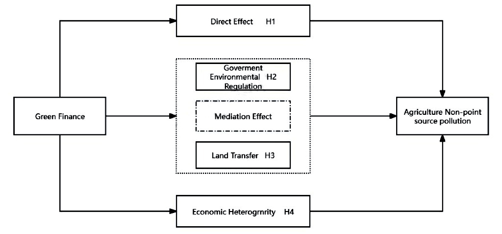
Based on the above assumptions, this paper constructs a theoretical model to examine the impact of GF on ANPSP. The model clarifies the intermediary roles of ER and LAND, as well as the influence of economic heterogeneity on ANPSP. The theoretical analysis of the model’s mechanism is illustrated in Fig 1.
Research Design
Basic Modeling Setting
Referring to the research of Jochmans and Verardi [33], based on the characteristics of agricultural economic activities and rural life, ANPSP primarily originates from pollutants generated during farmland cultivation. These pollutants include total nitrogen (TN), total phosphorus (TP), chemical oxygen demand (COD), carbon emissions, as well as pesticide and agricultural film residues. Organic matter and nitrogen-phosphorus pollutants often infiltrate surface water bodies through surface runoff and farm drainage, especially during precipitation or irrigation events. ANPSP measurement commonly employs an inventory analysis approach based on unit surveys, accounting for pollution from aquaculture, pesticides, and agricultural films. ANPSP is estimated from seven key sources: agricultural fertilizers, livestock and poultry farming, aquaculture, crop cultivation, rural population, pesticide usage, and agricultural films. Data for ANPSP surveys are primarily sourced from the State Environmental Protection Administration, the Second National Pollution Source Census, and the Statistical Yearbook. The framework for the basic model is outlined as follows:
Where: ANPSPit denotes the level of ANPSP emissions; GFit denotes the level of GF development; Controlsit is the set of control variables; σt denotes time-fixed effects; εit denotes the random error term; subscript i denotes the region; and subscript t denotes the year.
Mediating Effects Model
Building upon prior analysis, it is posited that GF can influence ANPSP both directly and indirectly through the promotion of ER and the facilitation of land transfer. Referring to the study by Hsiao et al. [34], this paper advances the Benchmark regression model (1) and model (2), aiming to explore the mediating roles of ER and land transfer degree in the nexus between GF and ANPSP. The specific formulation of the model is presented as follows:
In equations (2) and (3), lnMEDit denotes the mediating variables after taking the logarithm, including two variables of ER and the degree of land transfer. The rest of the variables are explained in the same way as in equation (1).
Variable Selection
Explained Variables
Agricultural production generates various forms of surface source pollution, predominantly consisting of total nitrogen (TN), total phosphorus (TP), chemical oxygen demand (COD), carbon emissions, and residues from pesticides and agricultural films. This pollution impacts the soil environment directly and also reaches water bodies through a combination of precipitation, topography-driven runoff (both surface and subsurface), and plant interception [35]. To measure agricultural pollution, this study employs the inventory analysis method based on unit surveys. This method encompasses pollution from both aquaculture and the use of pesticides and agricultural films. It estimates ANPSP across seven dimensions: agricultural fertilizers, livestock and poultry farming, aquaculture, crops, rural population, pesticides, and agricultural plastic films. The indicators used for this analysis are detailed in Table 1.
The emission intensity of ANPSP is calculated as:
In equation (4), the TE is the total emission of ANPSP; ETP, ETN, ECOD are the total emissions of total nitrogen (TN), total phosphorus (TP), and chemical oxygen demand (COD), respectively. In equation (5), the EUi is the statistic of the pollution unit i; ρi is the pollution production coefficient of the pollution unit; and θi is the emission coefficient or loss rate. The pollution intensity of various units differs due to distinct influencing factors. For the calculation of emissions from ANPSP, the coefficients for the seven pollution units are utilized as follows:
(1) Agricultural Fertilizers: The fertilizer pollution emissions = fertilizer application × loss coefficient. To account for variability in fertilizer loss rates across planting methods, this study applies the output coefficient method. Given that the Statistical Yearbook, recorded as phosphorus pentoxide (P₂O₅), is adjusted by 43.66%. Based on recent domestic fertilizer application practices and past research, compound fertilizers are discounted by 40% for TN and 32% for P₂O₅. The fertilizer loss coefficient is derived by averaging data from different regional studies, following methods from the second national pollution source census [36].
(2) Livestock and poultry farming. The pollution emissions are calculated as the product of the total quantity of livestock and poultry (either in stock or slaughtered), multiplied by both the pollution discharge coefficient and the wastage coefficient. The discharge coefficients for feces and urine of livestock and poultry are sourced from SEPA data (2022). The formula applied is: Livestock and poultry pollution intensity (kg per head per annum) = Rearing cycle × Fecal (urine) emission factor × Fecal (urine) pollutant excretion coefficient. In this study, livestock and poultry statistics encompass cattle, sheep, and pigs. For cattle and sheep, which have a rearing period of more than one year, the total breeding amount is based on the year-end stock.
(3) Aquaculture. ANPSP primarily arises from bait residues, aquaculture excreta, and chemicals. The extent of this pollution is contingent on the aquaculture type and method. The China Statistical Yearbook classifies aquaculture production into marine and freshwater categories. Given that artificial aquaculture is a significant pollution contributor, this paper exclusively utilizes data from freshwater aquaculture for its analyses. The primary aquaculture species include freshwater fish, crustaceans, shellfish, and other aquatic organisms. The production and discharge coefficients for aquaculture are derived from the First National Pollution Source Census: Handbook of Production and Discharge Coefficients for Pollution Sources in Aquaculture, supplemented by additional literature [37].
(4) Crops. The primary pollutants from crops include residues, vegetable wastes, and other debris from agricultural production [38]. Given the diverse range of crops, this paper focuses on the seven most representative ones for analysis: rice, wheat, maize, beans, potatoes, oilseeds, and vegetables. The estimation of surface source pollution from agricultural solid waste involves calculating the crop residue yield based on the grass to grain ratio and determining the total nitrogen (TN), total phosphorus (TP), and chemical oxygen demand (COD) content from the nutrient composition of the straw. Recognizing the varied straw utilization methods in rural areas, each with different nutrient loss rates, the final emission formula for farmland solid waste pollution is: Emissions (tons) = Total crop production (tons) × Production coefficient × Straw utilization structure × Straw nutrient loss rate, where the production coefficient equals the grass to grain ratio multiplied by the straw nutrient content [39].
(5) Rural domestic pollution is primarily divided into two categories: domestic sewage and human waste. For domestic sewage, the annual production coefficients per person are 5.84 kg for COD, 0.584 kg for TN, and 0.146 kg for TP, with an emission factor of 100%. For human waste, the annual production coefficients per person are 19.8 kg for COD, 3.06 kg for TN, and 0.64 kg for TP, with an emission factor of 10% [40].
(6) Pesticides. Pesticide residues are calculated as the amount of pesticides applied multiplied by a residue factor of 0.5.
(7) Agricultural film. The amount of agricultural film residue is determined by multiplying the quantity of agricultural film used by a residue factor of 0.1.
Explanatory Variables: Level of GF Development
GF primarily aims to adhere to market economy principles while focusing on building an ecological civilization. It employs a range of financial tools, including credit, securities, insurance, and funds, to foster energy conservation, reduce consumption, and achieve a harmonious balance between economic resources and the environment. In the realm of existing literature, methodologies such as principal component analysis, the entropy value method, and hierarchical analysis are commonly used to determine the weights of GF development indicators. Following the approach of Li et al. [41], this paper develops indicators in seven domains: green credit, green investment, green insurance, green bonds, green support, green fund, and green rights and interests. These indicators are then integrated using the entropy method to formulate a GF index, which assesses the level of GF development. For this assessment, raw data is initially standardized, followed by the computation of the indicators. The detailed measurement methodology is presented in Table 1.
Mediator Variables
Environmental regulation (ER). The selection of the ER variable follows the methodology of Chen et al. [43]. This approach utilizes the frequency of terms related to “environmental protection” in local government work reports compared to the total word count of the report as an indicator. A higher frequency indicates a stronger commitment to environmental governance, thus reflecting the intensity of ER and addressing endogeneity concerns. Relevant terms include ecology, green, low-carbon, pollution, energy consumption, emission reduction, sewage, sulfur dioxide, and carbon dioxide. As local government work reports are typically published early in the year, they predate and thus are not influenced by that year’s environmental conditions, further mitigating endogeneity issues.
Table 1.
Indicator set for ANPSP and GF.
Land transfer (LAND). this paper adopts the rate of agricultural land transfer (calculated as the total area of family-contracted arable land transferred divided by the total area of family-contracted arable land operated) as the proxy variable. This rate is an effective measure of agricultural land transfer levels and is widely used in inter-provincial level studies.
Control Variables
In alignment with existing literature, this study selects five indicators as control variables: economic development (GDP), industrial structure (STR), openness to external influences (OP), Urbanization, and High-quality agricultural development (HAD). Details of how the indicators are measured and the corresponding references are given in Table 2.
Data Sources
This study focuses on 31 provinces in mainland China, excluding Hong Kong, Macao, Taiwan, Diaoyu Islands, Sansha City, and other regions, using panel data from 2005 to 2021 for empirical analysis. The primary data sources include the CSMAR database, Wind database, Green Patent Database from the China ReseaChina Statistical Yearbook, China Environmental Statistical Yearbook, China Rural Statistical Yearbook, China Animal Husbandry and Veterinary Yearbook, National Costs and Revenues of Agricultural Products, China Regional Statistical Yearbook, and Agricultural Statistics. Missing values were addressed using linear interpolation, and to mitigate heteroskedasticity biases from data outliers, all variables were logarithmically transformed. The descriptive statistics for the empirical data are presented in Table 3.
Empirical Results and Analysis
Benchmark Regression Results
After calculating the correlation coefficients, it is noted that most variables exhibit significance at the 1% level, which is highly satisfactory. Additionally, the variance inflation factor (VIF) test for the regression variables yields a VIF of 7.88, indicating the absence of severe multicollinearity issues. For the multiple regression analysis in this study, the two-way fixed effects model is employed, and the benchmark regression outcomes are presented in Table 4. Analysis of column (1) of Table 4 reveals that the coefficient estimate of GF on ANPSP is significantly negative at the 5% significance level when no control variables are incorporated. This underscores the significant inhibitory effect of GF on the development of ANPSP, thereby validating hypothesis H1 of this paper. Subsequent examination of column (2) of Table 4 shows that the estimated coefficient of GF on ANPSP remains significant at the 5% level after the inclusion of the control variables of economic development (GDP), industrial structure (STR), openness to external influences (OP), Urbanization, and High- quality agricultural development (HAD), the estimated coefficient of GF on ANPSP remains significant at the 5% level at -0.311 after the inclusion of the control variables. This suggests that even after accounting for other influencing factors, GF continues to exert a notable negative influence on ANPSP.
Table 2.
Description of how control variables are measured.
Table 3.
Descriptive statistics of variables.
From the results of the control variables, STR has a significant negative effect on ANPSP with a coefficient of -0.296 and is significant at the 1% level of significance, indicating that changes in STR may inhibit the development of ANPSP. The coefficient of HAD is 0.427 and significant at a 1% level of significance, indicating that the promotion of high-quality agriculture can help to improve the performance of ANPSP. On the other hand, the coefficient of OP is not significant, implying that there is no direct correlation between the increase in the level of openness to the outside world and the mitigation of ANPSP. The possible reason for this is that the effect of opening up is not easy to be seen in the short term. The coefficient of Urbanization is -0.169, which is also statistically insignificant. Still, the trend suggests that the process of urbanization may have some inhibitory effect on the safe production of agricultural products. The reason behind this may be that the de-farming of land resources in the process of urbanization has led to the compression of the agricultural production base.
Tests for Mediating Effects
In the analysis of mediating effects, ER and LAND are selected as the mediating variables of GF and ANPSP [34]. Models (3) and (4) in Table 5 demonstrate the results of the mediating effect of ER. Model (3) is the regression result of GF on ER with a coefficient of -0.991, which is significant at the 1% significance level, indicating that when GF is enhanced, it significantly reduces the level of ER. Model (3) shows the regression result of ER on ANPSP, and its coefficient is 0.106, which is significant at 5% significance level, indicating that the enhancement of ER helps to improve ANPSP. This suggests that ER is a partial mediator, which validates hypothesis H2. The possible reason for the negative effect of GF on ER is that there is a lag in the market mechanism in transmitting the policy objectives of green finance, but the enhancement of ER can reduce the level of ANPSP, suggesting that the government should strengthen the regulation and protection of agri-environment to help achieve the SDGs.
Models (5) and (6) in Table 5 demonstrate the results of the mediating effect of LAND. Model (5) is the regression result of GF on LAND with a coefficient of 1.536, which is significant at the 1% significance level, indicating that the extent of land transfer increases with the enhancement of GF. Model (6) shows the regression result of LAND on ANPSP, and its coefficient is 0.059, which is significant at the 5% significance level, indicating that the increase in the degree of land transfer will negatively affect ANPSP. LAND is also a partial mediator, and the development of GF can indirectly negatively affect ANPSP by increasing the degree of land transfer, thus verifying Hypothesis H3. Although land transfer can improve the efficiency of land use, it may also negatively affect the environment in the absence of appropriate environmental protection measures and regulations, and future land policy development needs to consider appropriate environmental protection measures.
Table 5.
Mediating effect results.
Robustness Tests
In table 6, two machine learning methods are employed for robustness testing. First, the Random Forest (RF) method is used to test model robustness. As an ensemble learning algorithm, RF effectively addresses nonlinearity and complex feature interactions while minimizing overfitting by constructing multiple decision trees for prediction. The parameters are set as follows: training set ratio at 0.8, number of decision trees at 100, minimum samples per node split at 2, minimum samples per leaf node at 1, with sampling performed with replacement, and out-of-bag (OOB) testing used. Subsequently, robustness testing is conducted using the XGBoost method. XGBoost, a gradient-boosting algorithm, enhances model performance through iterative training of weak learners (e.g., decision trees) while mitigating overfitting via a regularization term. The parameters are configured as follows: training set proportion at 0.8, learning rate at 0.1, booster type set to “gbtree,” number of base learners at 100, tree maximum depth at 6, sampling rates for both samples and features at 1.0, L1 regularization factor at 0, and L2 regularization factor at 1.
The results for model (5) using Random Forest reveal a GF weight of 0.078 and an R² of 0.843, indicating strong explanatory power. The RF model demonstrates the negative impact of GF on ANPSP by repeatedly splitting and combining variables, remaining robust after accounting for time and regional effects. For model (6), XGBoost results show a GF weight of 0.055 and an R² of 0.833, also demonstrating high explanatory power. Through gradient boosting, XGBoost highlights the importance of GF in multiple dimensions during iterative optimization, while regularization prevents overfitting. The model remains robust after controlling for time and regional effects.
Heterogeneity Analysis
To investigate whether regional economic disparities influence the effectiveness of GF in mitigating ANPSP, this study calculated the average per capita GDP across 30 provinces within the sample year. By comparing each province’s total per capita GDP against the average value of 12,078.75, the sample was divided into two groups: high and low economic development. The high economic development group consists of ten provinces: Beijing, Tianjin, Shanghai, Jiangsu, Zhejiang, Fujian, Shandong, Hubei, Guangdong, and Chongqing. In contrast, the low economic development group includes twenty provinces: Hebei, Liaoning, Anhui, Jiangxi, Henan, Hunan, Sichuan, Shaanxi, Shanxi, Inner Mongolia, Jilin, Heilongjiang, Guangxi, Hainan, Guizhou, Yunnan, Gansu, Qinghai, Ningxia, and Xinjiang. The test results are presented in Table 7. A comparison of the size and significance of the estimated coefficients reveals that the impact of GF on ANPSP is only observable in regions with low economic development, where the effect is significantly positive. This suggests that GF may inadvertently contribute to the spread of ANPSP in less economically developed areas. This phenomenon may arise for several reasons: first, regions with lower economic development levels often rely on outdated technologies and traditional agricultural practices, which tend to be less environmentally friendly. Additionally, resource allocation mechanisms in these areas are relatively weak, limiting the effectiveness of green financial resources for emission reduction. Second, regions with lower economic development may experience shortcomings in environmental regulation and enforcement. Consequently, even with GF support, the impact of environmental protection measures may remain constrained [50].
Conclusions and Policy Implication
Conclusions
Given the well-established influence of GF on reducing industrial pollution emissions, this paper theoretically examines the direct impact and transmission mechanisms of GF on ANPSP. Using panel data from 30 Chinese provinces spanning 2005 to 2021, this study employs a panel fixed effects model and a mediation effect model to assess the multidimensional impact and mechanisms of GF on both industrial pollution emissions and ANPSP. Additionally, machine learning methods were utilized to validate the robustness of the research findings.
(1) GF has a significant inhibitory effect on ANPSP.
(2) GF achieves pollution control and emission reduction for ANPSP through mechanisms such as GE and LAND policies.
(3) Heterogeneity analysis reveals that the positive effect of GF on reducing ANPSP is predominantly observed in regions with lower levels of economic development.
Policy Implication
Based on these findings, the paper recommends the following actions:
(1) Financial products frequently act as the “active agents” within the financial system, with product and tool innovation playing a critical role in advancing GF to address ANPSP. Currently, while China’s financial market is growing rapidly, green financial products are still predominantly limited to green credit and green bonds, with minimal development in other innovative green finance instruments. Looking forward, China’s financial sector should harness technologies such as blockchain and big data to diversify green financial offerings, including green insurance, green securities, green funds, carbon finance, and carbon options. Such diversification is essential, but equal emphasis should be placed on mitigating the risks that come with the swift expansion of GF. As environmental protection and sustainable development become more embedded in public consciousness, the base of green investors and consumers is expanding. Financial institutions are encouraged to adopt strategies that prioritize “popularization, openness, and low barriers to entry,” leveraging internet platforms to broaden investor participation and integrate GF into daily life. Additionally, these institutions should deepen their strategic understanding of sustainable development, cultivating an environment where financial involvement in ANPSP management is viewed as a rational and sustainable choice. This approach supports the long-term development of both the financial and agricultural sectors.
(2) Strengthening environmental regulation is crucial for effectively mitigating ANPSP, especially through expanding and refining regulatory standards and scope. Presently, China’s environmental regulation relies significantly on Pigovian principles, aiming to balance individual earnings and social costs by curbing pollution’s negative externalities via taxation and promoting positive environmental outcomes through subsidies. However, in the agricultural sector, particularly in livestock breeding, the effectiveness of these regulations can be limited. For example, while policies encourage investment in waste recycling infrastructure, the ongoing use of such equipment may still present environmental risks. To address these challenges, environmental regulations should be precisely tailored to cover all potential pollution sources throughout the agricultural production chain. Taxation and subsidies should be carefully allocated to fit specific contexts, creating a balanced framework that maximizes environmental benefits. Additionally, regulatory policies must clearly define target entities, tailoring strategies to address the unique characteristics of individual farms and larger agricultural enterprises alike. Setting clear, overarching goals and structured processes for these regulations will enhance their impact on ANPSP reduction, fostering more sustainable agricultural practices.
(3) Given the positive impact of land transfer on pollution management, it is crucial to expand the scope of GF. Firstly, the GF system should facilitate the efficient flow and market-driven allocation of land resources, providing strong support for emerging sectors like the carbon sink economy, GF, and land bonds. Innovative financial products – such as green credit, green bonds, and green funds – should be developed to leverage natural resources like land. Tailored green credit support based on local requirements, the establishment of pilot trust zones, and improvements in land management systems are all necessary steps in this direction. Moreover, since financial institutions may have reservations about investing in rural land due to trust issues, we recommend initiating urban pilot projects to implement scalable land regulations. When financial institutions’ confidence in rural land investments strengthens, regulatory refinements can be made based on pilot feedback, thus minimizing risks tied to unstructured trust arrangements. Additionally, prioritizing the establishment of a comprehensive legal framework for rural land credit can lower access barriers to land credit, promoting effective land transfer policy implementation. This includes refining laws and regulations governing land operational and management rights and actively promoting land transfer to reinforce land-interest linkages. Such initiatives can encourage farmers to engage in land transfer, thereby fostering sustainable land management practices.
(4) To promote sustainable economic growth, regions with high economic development must prioritize ecological preservation to balance economic advancement with environmental protection. This focus helps prevent the “disorder effect” often linked to excessive resource consumption and cumulative pollution. For regions with lower economic development, policymakers should consider the challenges, or “pain points,” associated with transitioning to green practices. This transition requires restructuring traditional industries, optimizing economic frameworks, and addressing other transformative issues. Additionally, these regions should actively adopt advanced green technologies in agricultural production, such as precision agriculture and ecological planting. Chinese policymakers should address regional imbalances in environmental policies by fostering a coordinated approach to governance. This includes strengthening inter-regional connections in the creation and implementation of environmental laws and regulations and encouraging cross-sector and cross-regional collaboration for comprehensive governance. Moreover, national or central-level Chinese authorities should implement authoritative, scientifically grounded, and strategically guided policies to manage ANPSP. For example, establishing a dedicated environmental information-sharing platform would reduce regional disparities in data availability, thereby enhancing nationwide efforts to control agricultural surface pollution.