Soil Quality Improvement and ACE Reduction

Agriculture is generally regarded as the curse of ecological protection [36]. Agricultural production leads to the loss of wildlife habitat [37] and some regulatory services, such as carbon storage or soil erosion control [38]. Farmland soil carbon storage accounts for 8%-10% of land soil carbon storage. Because of natural factors and agricultural production activities, farmland soil is in a process of constant change. Long-term traditional farming combined with the overuse of agricultural chemicals degrades soil organic carbon storage [39]. The loss of soil organic carbon causes CEs resulting from the oxidation of the organic carbon after farming [40]. Some studies have shown that about 60%-70% of the above loss can be refixed, and the soil carbon pool can be increased by 0.4-0.9 PgC every year for 50 years, as estimated by the IPCC, with the aid of appropriate management measures. The cumulative increase in the oil carbon pool is 24-43 PgC [41]. HSBF involves better soil texture through soil improvements, increasing the thickness of the farmland tillage layer, ameliorating the soil and soil fertility by adopting agronomic, biological, and other measures, and promoting the content of soil organic matter by applying farmyard manure and returning straw to the field. Adding organic matter improves soil carbon status and sequestration, as well as soil quality [42]. In addition, through the promotion of conservation tillage, the saline alkaline soil, acidified soil, and heavy metal-contaminated soil can be controlled, the soil’s physical and chemical characteristics in the tillage layer can be improved, and soil pH can be maintained at 5.5- 7.5. The improvement of soil quality enhanced carbon sequestration on farmland and reduced ACEs. Moreover, soil improvement and soil fertility make farmland fertile, which reduces the application of fertilizer to a certain extent and promotes ACE reduction.

WRUE and ACE Reduction

China’s water resource scarcity and uneven spatial allocation of water resources. The HSBF construction policy also focuses on constructing agricultural water facilities and promoting water-saving irrigation technology. Nearly half of the farmland in China is without irrigation water or conditions, but the irrigation in some areas is flood irrigation, which seriously wastes water resources. Agriculture production activities both contribute to and are easily influenced by climate change [43]. The increase in climate extremes such as drought, heavy precipitation, and tropical cyclones has a huge impact on agricultural production and universal life. Climate change contributes to the increased probability and intensity of drought [44]. Drought causes food loss and affects food security. For areas with irrigation facilities, irrigated and non-irrigated farmland affects the unit grain yield, which is 1.67-1.89 times higher for wheat and 1.47-1.53 times higher for corn. Irrigation is crucial for stabilizing grain yields. China’s agricultural water supply accounts for 60%-70% of the total water supply [45]. Due to the growing demand for water, this results in a lack of surface water and the depletion of groundwater. CEs from the development and utilization of water resources are an important part of ACEs. CEs from irrigation account for about 22% of the total CEs from agricultural production [46]. Improving the WRUE can reduce the excessive consumption of water resources and CEs. Water-saving irrigation can reduce water consumption and improve the WRUE to reduce ACEs.

In view of the aforesaid analysis, we propose the following hypotheses: H1: The implementation of RLCP can reduce ACEs. H2: RLCP reduces ACEs by improving soil quality and WRUE.

DID Model

The DID model is the main method to estimate policy effects. The construction of HSBF is the most important element of the second phase of RLCP. HSBF was implemented nationwide in 2011, focusing on the major grain-producing regions and giving due consideration to other regions. Therefore, in different periods of the policy’s implementation, HSBF in each province differed in size and progress. The implementation year and regional heterogeneity of HSBF are such that RLCP can be regarded as a quasi-natural experiment. Here, we use the DID model to estimate ACEs resulting from RLCP. We use the identification strategy of continuous DID and the continuous variable of the “HSBF area ratio” to differentiate the experimental group (samples with a high HSBF area ratio) from the control group (samples with a low HSBF area ratio).

The continuous DID model is formulated as follows [48]:

Where ACEit is the ACEs of province i in year t, DID represents Hi×Itpost, equal to the proportion of the HSBF area ratio and the dummy variable at the time of RLCP policy implementation; Xit is a control variable, ui is the fixed effect of provinces; ζt is the fixed effect of time; εit is the random error term, α is the constant, and β and γ are the parameters to be estimated.

SDID Model

The implicit identified assumption of the DID method is that any individual in the collectivity will not be influenced by other individuals receiving the treatment (the stable unit treatment value assumption, SUTVA). This excludes the interaction between individuals and strictly assumes that individuals are independent of each other [49]. However, in the case of the RLCP, regions are subject to spillover effects. Due to the violation of the SUTVA hypothesis, the measurement method of the RLCP effect based on the SDID method needs to be further expanded. Contrary to the DID model, the SDID model relaxes the SUTVA hypothesis and considers the spatial spillover effects of RLCP.

The DID model can only evaluate the impact of RLCP on individual pilot regions. It ignores the test of spatial spillover effects, diminishing the robustness and authenticity of the results. Therefore, we constructed a SDID model to research the impact of RLCP on ACEs. The SDID model [50] can be expressed as follows:

Where ACEit, DID, α, β, γ, Xit, ui, ζt, and εit are the same as in Eq. (1); W is a spatial weight matrix (SWM); WDID is the reciprocal impact of DID on neighboring regions; and WACEit represents the spatial lag term of ACEs.

There are three spatial econometric models commonly used to estimate SDID models, namely the spatial Durbin model (SDM), the spatial autoregressive model (SAR), and the spatial error model (SEM). The SDM model can be simplified into SAR and SEM, and the most suitable model can be determined by a likelihood ratio (LR) test and the Wald test [51]. The SWM is the spatial distance between regions. According to the first law of geography, the spatial distance can also reflect the degree of interdependence between regions, which is the basis of spatial econometric analysis. According to the aims of our study, we established three SWMs for analysis:

Spatial Correlation

Before establishing the SDID model, it is necessary to use Moran’s I to analyze the spatial correlation of ACEs as the basis for evaluating the spatial spillover effects of RLCP policies:

where S2=1n∑i=1n(Yi−Y―)2, Y―=1n∑i=1nYi; Y represents the ACEs of province i; n represents the number of provinces; and W=(wij)n×n is the SWM. The value of Moran’s I is between -1 and 1, and the closer it closes to being 1, the stronger the positive spatial correlation is. On the contrary, the stronger the negative spatial correlation.

Moran’s I of ACEs

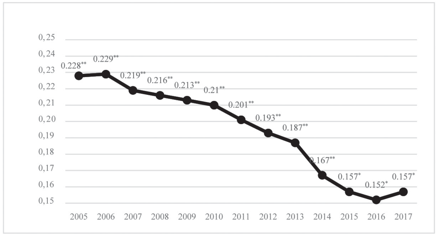
Before using the SDID model for empirical analysis, it is essential to prove the spatial correlation of ACEs. The global Moran’s I was calculated by the adjacency SWM (Fig. 1). We found that the global Moran’s I is significantly greater than 0, indicating that ACEs show significant spatial correlation characteristics. In addition, it showed a downward trend since 2006, a slow rise since 2016, and a slow downward trend in general. This means the spatial correlation of ACEs has gradually weakened from 2005 to 2017. Therefore, we constructed a SDID model for analysis.

Parallel Trend Testing

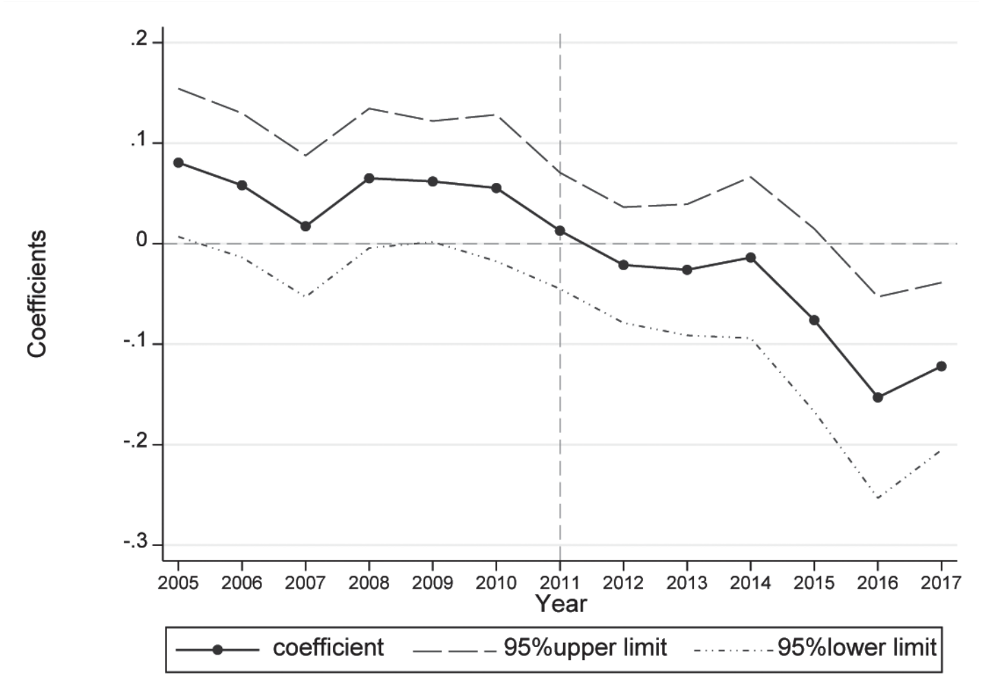
A fundamental assumption with the SDID model is that before the RLCP policy, ACEs in non-pilot areas and pilot areas had the same trend of change. Consequently, we used the event study method to verify whether this assumption was broken. Referring to existing research [52], we used the event study method to verify the dynamic effects of RLCP policy. Specifically, we replaced the DID variable in the benchmark regression with dummy variables representing several years before and after the implementation of RLCP and tested the parallel trend assumption based on the following equation:

Fig. 1.

Global Moran’s I from 2005 to 2017

where DID^k_it is a variable of the RLCP policy. Since the relevant data were updated to 2017, the data years after the implementation of the RLCP in the sample only include the six years from 2011-2017. Therefore, the threshold value of the virtual variable is set to 6. Let S_i be the implementation year of the RLCP policy, where k=t−Si,k∈[−6,6]. αk represents the impact of RLCP on ACEs. Fig. 2 depicts the 95% confidence interval of the direct effects under the geographical adjacency SWM. The horizontal axis is the year, and the ACEs have parallel trends in pilot and non-pilot. The results verify that the trend is stable in advance. Therefore, the RLCP can be seen as a quasi-natural experiment. Further, we found that the RLCP policy had a sustained inhibitory effect on ACEs. In the first three years, the impact of the RLCP policy on ACE reduction was relatively small, and in the fourth year, the impact became larger. However, the coefficient in the fifth year has an upward trend, but the impact still exceeds that in the fourth year.

Benchmark Model

RLCP had a negative impact on the total ACEs (Table 2), and the results were significant at the 1% level (Model 1). The coefficient of DID is -0.050, indicating that the implementation of the RLCP policy suppressed 5% of ACEs and had significant environmental effects. After that, the SDID was used for estimates. SWMs are the foundation of spatial econometric analysis, and different settings of weight matrices lead to different results, affecting the robustness of empirical analysis. We used adjacency weight matrices, geographic distance matrices, and geographic and economic distance nested matrices for spatial econometric analysis. We used the Lagrange multiplier (LM) test, the Hausman test, the LR test, and the Wald test to confirm the specific form of SDID. (1) Based on the LM and robust LM statistics, we inspected whether the SAR or SEM model was selected. If the LM test demonstrates that the model has spatial effects, they can be directly estimated using a more general SDM. (2) The Hausman test results were used to choose whether to use fixed or random effects. (3) We used the LR test to confirm whether the SDM contains time or spatial fixed effects. (4) Wald’s test was used to determine whether the SDM model would degenerate into the SAR or SEM model. According to the test results, we selected the SDM model with time and spatial fixed effects.

Fig. 2.

Parallel trend test

Models (2) to (4) demonstrate the estimation of the SDID model. It can be seen that the estimation results of the SDID model under the three SWMs are relatively consistent, indicating that the SDID model is relatively robust and trustworthy. The coefficients of DID are all negative, and they all pass the 1% significance test under the three SWMs. The results indicate that the RLCP has a significantly positive impact on ACEs. The coefficient of WDID is also negative, and it is uniform at the 5% significance level, demonstrating that the construction of RLCP may have a negative spatial spillover effect on ACEs and that the construction of RLCP in neighboring regions had a demonstrative effect on the region. Elhorst [53] specified that when global interaction effects are included in the model set, the point estimation results of the spatial econometric model do not typify the marginal impact of the independent variables. Accordingly, in order to compare and analyze the heterogeneity in the effect of each independent variable and its spatial spillover effects, it is essential to further calculate the direct and indirect effects of each independent variable based on the point estimation of the model.

Direct and Indirect Effects of RLCP

As mentioned above, there is a spatial dependence of ACEs in various provinces. In virtue of the existence of global interaction effects in the SDM, the coefficient of the DID variable cannot directly calculate its impact on ACEs. For the sake of better revealing the impact of RLCP on ACEs, this section decomposes the spatial effects, including the direct and indirect effects of RLCP on ACEs (Table 3). The coefficients of RLCP policy’s direct effects are negative under the three SWMs, with impact coefficients of -0.048, -0.071, and -0.052. The coefficients are all at the 1% significance level, proving that RLCP policies had a significant inhibitory effect on ACEs in the region and thus verifying hypothesis H1. RLCP promotes the rational use of land resources and the optimization and improvement of the land use structure. In order to increase production and income, agricultural operators unreasonably apply a large number of chemicals, such as fertilizers, resulting in increasingly barren land fertility and increasingly hardened plots. Due to resource endowments and technical constraints, individual farmers are unable to effectively improve soil quality, because poor soil fertility results in a large amount of chemical products being applied, falling into a cycle of increased poverty. RLCP can repair damaged cultivation layers through agronomic and biological means, improving the content of soil organic matter, thereby improving land quality, and promoting the reduced use of chemicals by agricultural operators to reduce carbon emissions. Moreover, the promotion of organic fertilizer and soil testing formula fertilization during construction plays a demonstrative role, guiding agricultural operators to rationally utilize land resources and scientifically input agricultural production factors to reduce ACEs. Due to factors such as climate change and irrational land use, water and soil erosion are relatively typical. In 2020, the area of water and soil loss reached 2.6927 million square kilometers, resulting in the loss of land productivity, siltation of watercourses, and pollution of water quality. The annual loss of nitrogen, phosphorus, and potassium fertilizers also caused enormous economic and ecological losses.

The indirect effects of the DID variable have a significantly negative impact under the three SWMs, indicating that RLCP policy can inhibit ACEs in surrounding regions and that the construction of RLCP not only directly affects ACEs in the local region, but also significantly inhibits ACEs in other regions through spatial spillover effects. Hypothesis H3 is thus verified. Compared to the adjacent SWM, the indirect effects of RLCP policy under the geographical distance SWM and the nested SWM are higher, indicating that policies in regions with closer geographical and economic distances generate more spatial spillover effects. The construction of RLCP also promotes the flow of productive factors such as technology, and it promotes the optimization of agricultural resource allocation in surrounding regions as well as ACE reduction. Regions with high levels of AGD can have demonstrative and competitive effects on surrounding regions. Regions with low levels of AGD can imitate and learn from regions with high levels of AGD, promoting the agricultural green transformation of the region. On the one hand, in the process of constructing the RLCP, there has been a gradual shift towards a green and ecological approach to farmland construction, shifting from a focus on production to one that emphasizes production and ecology equally.

The direct effect of Eco on ACEs has a negative and significant impact under the three SWMs, indicating that regional economic development can suppress local ACEs, while the indirect impact of Eco on ACEs is positive and significant. The development of the regional economy promoted an increase in ACEs in neighboring provinces. The higher the level of economic development in a region, the more the public will increase demand for agricultural green food. This motivates agricultural operators to use greener and more environmentally friendly production methods and reduce ACEs. The direct, indirect, and total effects of the market variable on ACEs are significantly negative, indicating that regional marketization promotes the reduction of ACEs. The direct and indirect effects of the Mech variable on ACEs are significantly positive, illustrating that the Mech promoted local ACEs, while the cross-regional operation of agricultural machinery also promoted ACEs in surrounding regions. The direct effect of the Income variable on ACEs is positive and significant. One reason for this is that the increase in farmers’ income mainly came from an increase in non-agricultural income, while non-agricultural industrialization led to a disorderly increase in agricultural chemicals.

Set Virtual the Time of RLCP Policy

Previously, we stipulated a binary dummy variable of 2011 as the RLCP policy time point. For the sake of robustness, we randomly selected the years 2007 and 2008 as the time of the RLCP policy for placebo estimations. As shown in columns 1 and 2 in Table 4, when 2007 and 2008 are taken as the RLCP policy time points, the coefficients of the DID variable are -0.013 and -0.014 and not significant, indicating that the policy time points are not random and that the estimated results are reliable.

Eliminate Other Policy Interference

After the New Development Concept was proposed in 2015, with “green” as one of the five major development concepts, the concept gradually permeated the agricultural field. In particular, corresponding agricultural policies such as the zero-growth action of fertilizer and pesticide and the reduction and efficiency of fertilizer and pesticide (as proposed in 2015) inevitably had an impact on ACEs. Therefore, we excluded samples from 2015 and beyond to eliminate the impact of other policies.