

Introduction
Global carbon emissions and economic growth have strongly correlated since the 1970s. Carbon and per capita emissions have increased dramatically with global economic development, resulting in regular climate anomalies and major climate disasters worldwide; therefore, addressing global climate change has become a common concern for humanity. At the 26th UN Climate Change Conference of the Parties (COP26) in 2021, the United Nations proposed that global carbon emissions would peak in 2030, although reduction efforts are still insufficient. China, the second largest economy in the world, cannot be left alone in the face of the grave global climate change crisis.
China has maintained medium-to-high-speed economic growth since its reform and opening-up, but at the same time, numerous adverse effects, such as the energy crisis and environmental pollution, have been brought about. Global attention and action have been focused on sustainable development, especially the greenhouse effect caused by a large amount of CO2 emissions. As the world’s second-largest economy and the largest manufacturing and foreign trade country, China completed the climate action goals set in the Paris Agreement by the end of 2019, highlighting the responsibilities of a great nation. At the general debate of the 75th session of the UN General Assembly in 2020, China committed to peak carbon dioxide emissions by 2030 and achieve carbon neutrality by 2060 (referred to as the “double carbon” goal). To achieve the “double carbon” goal as soon as possible, carbon emission reduction in secondary and tertiary industries is critical, and as a necessary “carbon source,” agriculture should not be left out of the picture. China is in a critical period of building agricultural and rural modernization, and agricultural development still relies heavily on factor drive. Therefore, promoting the rapid development of agriculture will exacerbate CO2 emissions to a certain extent. In order to explore more effective ways to reduce agricultural emissions, more and more scholars have started to conduct relevant research on agricultural carbon emissions in recent years and formed fruitful research results, which mainly focus on two aspects.
First, a large and growing body of literature has investigated the measurement, evolution, and influencing factors of agricultural carbon emissions. In terms of measurement and evolution, it is found that agricultural irrigation is emphasized as one of the primary carbon sources. China’s total agricultural carbon emission shows an overall cyclical upward trend but at a markedly slower pace [1, 2]. With the deepening of research, the measurement and evolution of agricultural carbon emissions have gradually expanded from the time dimension to the spatial dimension. An investigation into the spatial dimension found that the agricultural carbon emission intensity is spatially aggregated in China, with significant differences between regions [3]. In terms of influencing factors, factors such as digital transformation, green finance, and production efficiency have a significant impact on agricultural carbon emissions [4-7].
Second, more recent attention has focused on providing carbon emission reduction. Although carbon emission reduction has become a consensus, according to the current development trend, the targets agreed in the United Nations Framework Convention on Climate Change (UNFCCC) will be challenging to achieve. Research has found that the synergy between taxation and other policies is beneficial for reducing carbon emissions in food consumption [8]. However, as a significant “carbon reduction” policy, there is still controversy over whether a carbon tax should be levied on China, as imposing a carbon tax solely on agriculture will reduce its competitiveness, and carbon emissions will not significantly decrease [9]. In addition to tax means, agricultural technological progress can promote agricultural carbon emission reduction [10], and achieve the targets of reducing greenhouse gas emissions by optimizing the planting structure and rotation system [11]. However, whether technological progress can play a role in agricultural carbon emission reduction is affected by other factors, such as the degree of opening up to the outside world [12]. At the same time, due to globalization, China’s agricultural trade impacts the agricultural carbon emissions of countries along the Belt and Road [13].
To sum up, the market regulation mechanism of China’s agricultural carbon emissions needs to be improved, and the cyclical upward trend of total agricultural carbon emissions has yet to be reversed. One important reason is that the agricultural input structure needs to be sufficiently optimized. Given the role of negative externalities, if environmental regulatory-related measures are not restricted, the private sector’s investment in agricultural productivity is higher than that in clean energy and carbon emission reduction [14]. Therefore, government intervention plays a vital role in promoting agricultural carbon emission reduction, leading some scholars to focus on the impact of government intervention.
Investment in clean agricultural energy and other public products cannot be separated from the government’s guidance, but fiscal stimulus may promote carbon emission reduction and trigger a carbon lock-in effect. Some studies have found that Chinese-style fiscal decentralization will lead to environmental deterioration [15]. When the government faces financial constraints, it will lead to insufficient public investment and reduce environmental supervision standards to a certain extent [16], which in turn indirectly leads to environmental deterioration through two channels: environmental supervision and industrial transformation, resulting in a “green paradox” [17]. Therefore, an essential prerequisite for China’s fiscal decentralization system to promote carbon emission reduction is continuously increasing the per capita fiscal investment and keeping the fiscal investment above a certain level [18]. However, some studies have also pointed out that local governments in China prioritize economic development over environmental protection and carbon control, and fiscal decentralization has no significant regulatory effect on environmental regulation and carbon emissions. Government spending can worsen environmental quality [19, 20].
The above literature review makes it easy to find that the existing research has provided relatively affluent findings on agricultural carbon emissions, laying a solid foundation for the follow-up, in-depth discussion. However, there are also some limitations: first, there needs to be more literature to systematically investigate the relationship between fiscal expansion and agricultural carbon emissions in the agricultural field. Thus, conducting an in-depth analysis of this critical issue from a theoretical perspective is necessary. Second, the relationship between fiscal investment and environmental quality has not reached a unified conclusion. As the core industry of the national economy, agricultural fiscal investment must strike a more careful balance between development and emission reduction, and the applicability of existing research conclusions to agriculture remains to be seen. Third, the existing literature needs to consider the macro environment’s regulatory role in investigating the effect of fiscal investment on carbon emission reduction. With this in mind, this paper attempts to build a theoretical analysis framework for analyzing the impact of fiscal expansion on agricultural carbon intensity based on externality theory and public goods theory to analyze further the possible impact of fiscal expansion on the total amount of agricultural carbon emissions and consider the realistic macro-environmental factors such as economic growth pressure, market segmentation, and industrial structure, ultimately explain the agricultural carbon emission effect caused by China’s fiscal expansion from both theoretical and empirical aspects.
The rest of this paper is arranged as follows: the next section is theoretical analysis; in section 3, we introduce the main research methods and data sources; in section 4, we report the main empirical results; section 5 is the conclusion and recommendation.
Theoretical Framework and Research Hypothesis
Compared with the secondary and tertiary industries, agriculture has its particularity. The main differences are as follows: On the one hand, as the foundation of the national economy, the maintenance of food security is a fundamental issue related to the survival of a country and indeed of the world. Ensuring the stable growth of agricultural output is not only a hard constraint on the prosperity and development of population and economy but also one of the essential political tasks of the government [21]; on the other hand, agriculture has the dual attributes of being a carbon source and a carbon sink [22]. The primary way for the agricultural system to enable China’s “double carbon” goal is to develop green and low-carbon agriculture with low energy consumption, low pollution, and low emission, as well as to realize a reduction in carbon emission and increase in carbon sink. Promoting the low-carbon transformation of agricultural production urgently needs a comprehensive balance between economic development and emission reduction.
Externalities occur when the impacts of market transactions are only partially reflected in prices. Externalities may be positive or negative. Positive externalities denote beneficial effects on third parties, whereas negative externalities signify adverse effects. Governments can address externalities by implementing taxes, subsidies, and regulations. For instance, implementing pollution taxes on companies emitting pollutants is a means of rectifying negative externalities. Public goods are characterized by non-excludability and non-rivalry, meaning that one person’s consumption does not impede others and is not efficiently provided through market transactions. Government intervention, typically through taxation or other financial support, is often required to furnish public goods, thereby safeguarding societal welfare. Theories on externalities and public goods are crucial frameworks for tackling market failures. These theories guide governments to implement appropriate policies to rectify market failures and enhance social welfare.
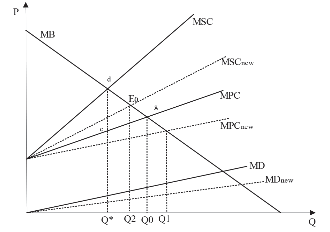
Carbon emissions are a common type of economic externality. The intensification of global carbon emissions is a notable manifestation of market failure. The externalities of agricultural carbon emissions are described in Fig. 1. The horizontal axis represents agricultural output Q, the vertical axis represents the price P, the curve MB represents the marginal income at each production level, MPC represents the private marginal cost corresponding to each output, MSC represents the social marginal cost corresponding to each output, MD represents the marginal damage caused by carbon emissions at each agricultural production level. From the private perspective, the profit maximization condition of private production is that the marginal cost is equal to the marginal income. That is, when MB is greater than or equal to MPC, production will be carried out. If MB is less than MPC, production will be abandoned. The maximum output is located at the intersection E0 of MB and MPC. The equilibrium output level of private production is Q0. From the social perspective, the best output is at the intersection of the social marginal cost MSC and marginal income curve MB. At this time, the best output is Q*. The social marginal cost MSC includes the private marginal cost and the marginal damage MD, so MSC = MPC + MD. As can be seen from Fig. 1, due to MSC also includes marginal damage MD, so Q* < Q0. Through the above analysis, the following conclusions can be obtained: first, due to the negative externalities of agricultural production (In fact, agricultural production also has positive externalities, such as providing more agricultural products for the society, supporting other industries, protecting the ecological environment, inheriting social farming culture, and so on), the private production market does not always equal the level of output that is socially efficient; in fact, the level of private production output is higher than the level of socially efficient output. Reducing agricultural carbon emissions to zero is generally not an ideal state of society. It is necessary to comprehensively weigh its production income and determine the optimal social output requirements.
Impact of Fiscal Expansion on Agricultural Carbon Intensity
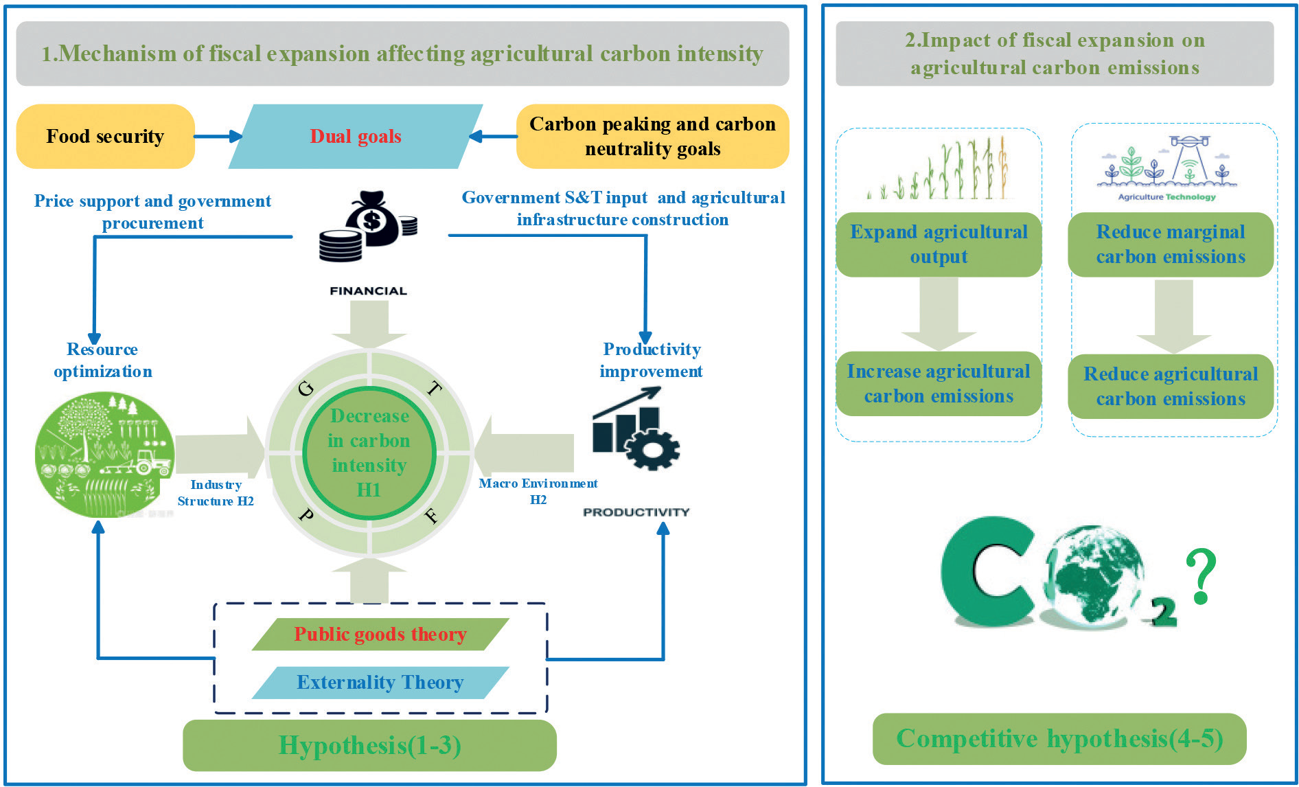
In the world’s emission reduction commitments and practices, carbon emission intensity and total carbon emission are two commonly used emission reduction indicators. In conjunction with Fig. 1 and 2, this paper discusses the impact of agricultural financial expansion on agricultural carbon intensity. China’s agricultural fiscal investment is generally spent in the form of national support projects (including agricultural infrastructure construction fees, science and technology fees, and utility expenses) and supporting agricultural production (including fiscal subsidy of infrastructure construction and production subsidy in line with the “green box policy” and so on). Therefore, expanding agricultural fiscal investment may reduce agricultural carbon intensity in two ways.
First, the productivity improvement effect. Based on public goods theory, fiscal expenditure can effectively supplement the inadequate supply of agricultural public goods, especially by supporting and guiding agricultural science and technology research, then exploiting the technical effect, which is conducive to generating knowledge spillover, to promote the capacity of agricultural regional technological innovation (including research and development of agricultural green and low-carbon technology, innovation of production means, scientific and technological progress), and to enhance the potential for sustainable reduction of agricultural carbon intensity. Furthermore, the non-competitive, non-exclusive, and non-divisive nature of agricultural infrastructure determines that it belongs to public goods and that the government generally provides pure public goods. Therefore, constructing agricultural infrastructure is a sizable component of agricultural fiscal expenditure. The improvement of agricultural production infrastructure is conducive to reducing the transportation cost of agricultural products, as well as agricultural input intensity, and popularizing electric agricultural machinery. Additionally, it promotes the agglomeration of agricultural industries to realize resource sharing and form centralization, which makes it easy to form a closely related specialized division of the labor system; besides, it saves transaction costs, produces positive spatial externalities, exploits the scale effect, improves productivity and reduces agricultural carbon intensity.
Second, resource allocation effect. Based on externality theory, because of the negative externality of carbon emissions, the market will have an excessive allocation of resources, and state intervention has become critical to compensate for the excessive allocation of market resources. Specifically, it affects in two ways: On the one hand, state intervention reduces the balanced output of private production by providing pollution subsidies to some polluting enterprises to reduce agricultural carbon intensity. On the other hand, the government supports and guides social capital to enter the field of agricultural green technology innovation through government purchases, provides agricultural public welfare technical services (farmers’ technical training, agricultural technology promotion, and moderate agricultural scale operation), improves the agricultural socialized service system, constructs a modern agricultural management system and upgrades the structure of the agricultural industry, finally optimizes resource allocation.
To sum up, fiscal expansion may improve agricultural green total factor productivity (GTFP) through the productivity improvement effect and resource allocation effect, so that the curve MD in Fig. 1 moves downward to the right to form a new curve MDnew, which implies a reduction in marginal damage. Other things being equal, fiscal expansion is conducive to reducing agricultural carbon intensity. However, everything has two sides. Although government intervention may further optimize the allocation of resources, excessive and improper government intervention may interfere with the fundamental decisive role of the market in determining resource allocation, which leads to a negative effect. Therefore, from a longer cycle, there may be a U-shaped nonlinear relationship between fiscal expansion and agricultural carbon intensity. According to the above analysis, this paper presents the research hypothesis 1–2.
Hypothesis 1: Fiscal expansion reduces agricultural carbon intensity by enhancing total factor productivity in agriculture.
Hypothesis 2: A U-shaped nonlinear relationship between fiscal expansion and agricultural carbon intensity.
Fiscal investment has long been a significant means of government intervention. The central government has created environmental protection incentives for local governments through fiscal transfer payments to improve local government’s environmental regulatory standards and reduce the environmental pollution of agricultural production to achieve the policy effect of reducing agricultural carbon emissions. At the same time, under the “combination of unification and decentralization” Chinese fiscal decentralization system, local governments have significant discretion in fiscal expenditure and resource allocation. The Chinese government passed two major fiscal decentralization reforms in 1979 and 1994, forming a governance model with Chinese characteristics through economic and political centralization. As a result, the field and structure of local government agricultural fiscal expenditure are influenced not only by the policy guidance of the central government’s transfer payment but also by a variety of other factors such as local government behavior, industrial structure, economic growth pressure, and so on. First, the market mechanism plays a decisive role in resource allocation; in contrast, fiscal expenditures’ direct role is to correct market failure. When the region is confronted with severe local protectionism, especially for the negative externality of environmental pollution, the excessive market segmentation led by the local government may cause the issue of excessive allocation of market mechanisms and fail to play its proper role in resource allocation. Second, the degree of rationalization of industrial structure varies significantly between regions. Since agricultural productivity in all parts of China lags behind the secondary and tertiary industries, the role of the market regulation mechanism is limited, and it is not easy to achieve the carbon emission reduction goal solely relying on the market strength. At this point, state intervention may result in more effective outcomes. Finally, since 2005, the Chinese government has started the pilot work of green GDP with the Environmental-Economic Accounting (SEEA) system as the investigation contents and changed the assessment system of officials based on GDP. Until 2016, the evaluation and assessment methods of the ecological civilization construction target issued by the CPC Central Committee’s general office and the State Council’s general office required Chinese officials to assess the environmental weight exceeded GDP for the first time. Under the rigid constraints of environmental assessment, an excessively high economic growth target may aggravate the local government to achieve the corresponding economic green growth target through fiscal expansion. Therefore, under the higher pressure of economic growth, the local government will have a more robust power to reduce agricultural carbon intensity through fiscal expansion. Based on the above analysis, this paper puts forward hypothesis 3:
Hypothesis 3: Fiscal expansion facilitates a reduction in agricultural carbon intensity. This reduction, however, is constrained by market segmentation, the degree of industrial structure rationalization, and economic growth pressure.
Hypothesis 3–1: Higher levels of market segmentation make fiscal expansion more favorable for reducing agricultural carbon intensity.
Hypothesis 3–2: Lower levels of industrial structure rationalization make fiscal expansion more favorable for reducing agricultural carbon intensity.
Hypothesis 3–3: Higher economic growth targets make fiscal expansion more favorable for reducing agricultural carbon intensity.
Impact of Fiscal Expansion on Total Agricultural Carbon Emissions
Based on the analysis of Fig. 1 and Fig. 3, it is found that fiscal expansion may reduce marginal damage MD. At the same time, another role of fiscal subsidies and technological progress is to reduce the marginal cost of private production, promote the curves MSC and MPC to move to the lower right at the same time, and form new curves MSCnew and MPCnew. The latest social optimal output increases from Q* to Q2,the increased agricultural output is Q2 – Q*, and the private optimal output also increases from Q0 to Q1. The economic implications of the above analysis is that fiscal expansion may expand the scale of agricultural production and increase agricultural output. Due to the positive correlation between output and agricultural carbon emissions, fiscal expansion may also have the effect of increasing the total amount of carbon emissions, which is MD × (Q2 – Q*). Based on our findings in the previous section that fiscal expansion has an emission reduction effect, assuming that the rate of marginal damage reduction caused by fiscal expansion is T, the total carbon emission reduction effect is expressed in T × MD × Q2. When MD × (Q2 – Q*) > T × MD × Q2, fiscal expansion will reduce the total agricultural carbon emissions; when MD × (Q2 – Q*) > T × MD × Q2, fiscal expansion will increase the total agricultural carbon emissions; when MD × (Q2 – Q*) = T × MD × Q2, the carbon emission increase and carbon emission reduction effect of fiscal expansion offset each other. From the above analysis, we can deduce that the impact of fiscal expansion on total agricultural carbon emissions mainly depends on the relationship between the increasing rate of fiscal expansion and the declining rate of agricultural carbon intensity. Therefore, fiscal expansion may increase or reduce total agricultural carbon emissions, that is, the relationship between fiscal expansion and total agricultural carbon emissions is uncertain and needs to be tested by empirical experience. As for the total amount of agricultural carbon emissions, the following two competitive hypotheses are put forward:
Hypothesis 4: Fiscal expansion reduces the total amount of agricultural carbon emissions.
Hypothesis 5: Fiscal expansion increases the total amount of agricultural carbon emissions.
Material and Methods
Study Area and Data Sources
Our final sample involves 30 provincial-level administrative regions (excluding Tibet, Hong Kong, Macao, and Taiwan). This paper uses the panel data at the provincial and regional levels from 2005 to 2021 for empirical analysis.
The data for measuring agricultural carbon intensity, total carbon emissions, total factor productivity, industrial structure deviation, market segmentation index, and relevant control variables were obtained from the China Rural Statistical Yearbook. The fiscal investment data of various regions are derived from China’s Finance Yearbook (http://www.stats.gov.cn/), and the economic growth rate targets of various regions over the years are derived from the government work reports of various regions. In order to eliminate the effect of magnitude between variables, all data are analyzed with standardized data.
Calculation of Total Agricultural Carbon Emissions
According to international greenhouse gas accounting systems such as ISO 14064 and GHG Protocol, emission sources are divided into three different ranges, namely direct emissions, indirect emissions, and other indirect emissions, to avoid the problem of large-scale double counting. This method is widely used internationally. This article is based on international standards, combined with the difficulties in data collection in China’s forestry carbon sink function and fishery carbon emission calculation. In addition, concerning previous literature [23], it aims to construct a carbon emission calculation system from the following three aspects: (1) Carbon emissions from agricultural materials and farmland production process, including indirect power consumption such as pesticides, chemical fertilizers, agricultural film, diesel, and agricultural machinery energy; (2) Methane (CH4) emissions in the whole growth process of rice; (3) Methane (CH4) and nitrous oxide (N2O) emissions from the intestinal fermentation of cattle, sheep and other livestock in animal husbandry and the management of their manure. As a result, the calculation formula for agricultural carbon emission is constructed as follows:
In the above formula, Ct represents the total agricultural carbon emission in year t, Cit represents the carbon emission of type i carbon source in year t, Tit represents the quantity of type carbon source in year t, and αi refers to the carbon emission coefficient of type i carbon source.
Calculation of Agricultural Green Total Factor Productivity
This paper constructs the production frontier surface based on the investigation period of all decision-making units (DMUS). Then, the agricultural green total factor production (AGTFP) is constructed using labor, land, and capital as input factors, agricultural output value as desired output, and carbon emission as unexpected output. Finally, the global Malmquist- Luenberger (GML) index is expressed as follows:
In the above formula, DTG(x, y, b) = max{β|(y + βy, b – βb ∈)pG(x)} is obtained according to the global benchmark production possibility set pG. Therefore, GMLt, t+1 > 1 indicates that AGTFP increases, GMLt, t+1 > 1 indicates that AGTFP decreases.
Table 1.
Descriptive statistical analysis.
Calculation of the Degree of Market Segmentation
The degree of market segmentation is measured by the average of the relative price variance of the consumer price index between a province and other provinces. Based on the “glacier” cost model, the market segmentation index is calculated by three-dimensional data of year, province, and commodity. The commodity price is the chain price index of regional commodities, and the calculation formula of relative price is:
In the above formula, i represents the region, t represents the time period, k represents the commodity type, P represents the price,
qitj is the relative price of goods after removing heterogeneity. Next, calculate the relative price variance (namely market segmentation index msegkt) for the combined relative prices of all adjacent provinces in region in period . When the market segmentation index is larger, it means that local protectionism is more serious.
Deviation Degree of Industrial Structure
Economic imbalance is a normal state, especially in developing countries. Hence, when analyzing the impact of fiscal expansion on agricultural carbon emissions, the effect differences under different industrial structures need to be considered. The deviation index of industrial structure measures the aggregation quality among industries, which reflects the degree of coordination between industries and the effective utilization of resources. The calculation formula is as follows: n Yi/Li – 1 n Yi/Y – 1
E represents the deviation index of industrial structure, Y represents the output value, L represents the number of employees, i represents the number of industries, and n represents the number of industrial sectors.
Model Setting
In order to accurately identify the relationship between fiscal expansion and agricultural carbon emissions, this paper uses a two-way fixed effect model for the empirical test. The specific model form is written as follows:
Where i represents the region and t represents the year. The dependent variables Aciit and Aceit respectively represent the agricultural carbon intensity and total agricultural carbon emission in phase t of the region i. FE represents the core variable fiscal expansion, and Xit is a series of control variables. According to the previous research, the control variables we selected include agricultural fixed asset investment, economic development level, urbanization level, agricultural economic development level, agricultural industrial status, agricultural industrial structure, and agricultural opening-up level. μi in the equation represents the unobserved factors related to a specific region, which is used to control for unobserved, time-invariant variability across provincial areas; μt refers to the year effect, which is used to control the economic development trend and changes in the macro environment faced by all regions; εit represents random disturbance term; Z means to standardize the original data.
Results and Discussion
Baseline Regression
Table 2 reports the results of the baseline model estimation of the impact of fiscal expansion on agricultural carbon emissions, where column (1) shows the estimated results of fiscal expansion on agricultural carbon intensity, and column (2) shows the regression results of fiscal expansion on total agricultural carbon emissions. The regression results in column (1) show that the coefficient of the fiscal expansion variable is -0.244 and passes the significance test at the 1% level, indicating that when the intensity of fiscal support to agriculture increases by one standard deviation, the agricultural carbon intensity will decrease by 0.244 standard deviations. This also means that appropriate fiscal expansion can promote the decrease of agricultural carbon intensity. Meanwhile, the coefficient of the squared term of the fiscal expansion variable is positive. Also, it passes the 1% significance level test, indicating that there is a type of U-shaped nonlinear relationship between fiscal expansion and agricultural carbon intensity; that is to say, excessive state intervention is not conducive to reducing agricultural carbon intensity after the proportion of fiscal support to agriculture reaches a certain intensity. There are two possible reasons for this. Firstly, in terms of economic growth, public finance theory points out that the macro resource allocation effect depends on the public sector of the government economy. If the scale of fiscal expenditure is large, it means that the public sector takes up too many resources in resource allocation, and the increase in government consumption reduces the macro resource allocation efficiency which is not conducive to economic growth, which is one of the possible reasons for the increase in carbon intensity. one of the reasons; secondly, in terms of carbon emissions, although the expansion of the scale of fiscal spending by the government as a provider of public goods is beneficial to reduce environmental pollution, China implemented a decentralized fiscal system after 1994. Excessive fiscal decentralization may intensify carbon emissions by intensifying fiscal and economic competition among local governments, and reducing environmental efficiency.
Table 2.
Baseline model regression results.
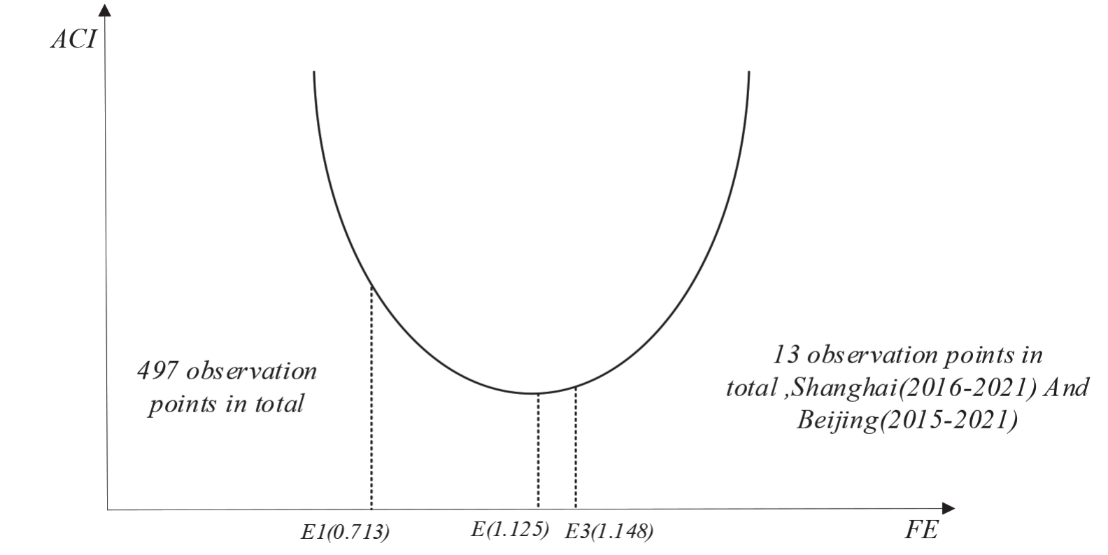
Fig. 3.
The relationship between the intensity of financial support to agriculture and agricultural carbon intensity type.
The results in column (2) show that although the coefficient of the fiscal expansion variable is positive, the coefficient of the squared term of fiscal expansion is negative. This indicates that there may be an inverse U-shaped relationship between fiscal expansion and total agricultural carbon emissions; in other words, fiscal expansion may promote the increase of total agricultural carbon emissions before they increase to a certain intensity, and fiscal expansion favors a reduction in total agricultural carbon emissions after it exceeds a certain intensity. The above explanation is in line with our empirical analysis, but surprisingly, neither the relationship between agricultural carbon emissions and fiscal expansion variable nor the relationship between agricultural carbon emissions and squared term of fiscal expansion variable pass the significance level test, and there is no statistically significant relationship between fiscal expansion and total agricultural carbon emissions, indicating that the relationship between fiscal expansion and total agricultural carbon emissions is uncertain.
Further, since there is a nonlinear U-shaped relationship between fiscal expansion and agricultural carbon intensity, after computational analysis, as shown in Fig. 3, the turning point of the U-shaped relationship between fiscal expansion and agricultural carbon intensity is around 1.125. On the right side of the turning point are 13 observation points, namely Shanghai (2016-2021) and Beijing (2015- 2021). The intensity of fiscal support for agriculture in these 8 observation points is greater than or equal to 1.148; that is to say, the regional fiscal expenditure on agriculture is more than 1.148 times the output value of the primary industry. Thus, the intensity of fiscal support for agriculture is significant. On the left side of the turning point are 497 observation points, and the fiscal support intensity of these observation points is less than or equal to 0.713. The average fiscal support intensity of all regions in China is only 0.208, which means the fiscal support intensity of most regions cannot reach the intensity of the turning point. Therefore, in China’s current low agricultural fiscal investment context, moderate fiscal expansion is conducive to promoting the decline of agricultural carbon intensity. At the same time, excessive state intervention is not conducive to promoting the decline of agricultural carbon intensity.
Heterogeneity Analysis
The impact effects of technology adoption and factor allocation are spatially heterogeneous [24], significantly, since the adoption rate of agricultural green technology differs between the prominent grain-producing areas and non-main grain-producing areas [25]. According to the national policy, this paper divides the country into main grain-producing areas and non-main grain-producing areas, among which the main grain-producing areas include 13 provinces and regions, including Hebei, Inner Mongolia, Liaoning, Jilin, Heilongjiang, Jiangsu, Anhui, Jiangxi, Shandong, Henan, Hubei, Hunan, and Sichuan. The main grain-producing areas produce about 75% of the country’s grain on 39% of the land, which is the key to ensuring basic grain self-sufficiency and absolute food security. For this reason, the central government has increased its support for the main grain-producing areas, proposing policies including raising the incentive standards for large grain-producing counties, focusing on rewarding large grain-producing provinces, and increasing subsidies for farmers to grow grain in the main grain-producing areas. Because of the different fiscal support regimes and food production pressures faced between main and non-main grain-producing areas, fiscal expansion may not have the same effect on agricultural carbon intensity between the two areas.
Table 3.
Estimation results for different regions.
The empirical estimation results based on different prominent and non-main grain-producing areas are shown in Table 3. The results show that fiscal expansion has positively promoted the decline of agricultural carbon intensity in non-main grain-producing areas. However, its impact on the decline of agricultural carbon intensity in non-main grain-producing areas is not obvious. There are three possible reasons for this: first, due to the hard constraint of national food security, the main grain-producing areas maintain the highest rate of agricultural production increase in the country, which also means that they are under greater pressure to reduce agricultural carbon emissions. Second, although sustainable soil and water management in agriculture and integrated rice farming in the main production areas are conducive to “carbon sequestration” and “carbon reduction” [26], in the main grain-producing areas, income from agricultural production is the primary source of income for most farmers, and farmers have a stronger incentive to increase food output by increasing the intensity of fertilizer and pesticide application. In addition, the weakness of agriculture determines its strong dependence on land and the natural environment, making it difficult for governments in main grain-producing areas to balance food security and agricultural carbon emission reduction. Together, the two weaken agricultural fiscal expansion’s carbon emission reduction effect. Third, the intensity of fiscal support in the main grain-producing areas must match the industry’s status. It is calculated that the average intensity of fiscal support for agriculture in the main grain-producing areas is only 11.35%, while the average intensity for agriculture in non-main grain-producing areas reaches 28.06%. Although the state has increased its financial support to the main grain-producing areas, more is needed.
Mechanism Test
In this study, fiscal expansion facilitates the reduction of agricultural carbon intensity, and there are significant differences across regions. Then, how exactly does fiscal expansion affect regional agricultural carbon intensity, and what is the specific mechanism of its effects? We will conduct detailed econometric tests based on the mediation model to answer these questions. Combining the ideas of the mediation model, we construct the following three regression equations.
Table 4.
Test results of influence mechanism.
Where the subscripts i and t denote the region and year, respectively; similar to the previous section, GTFPit denotes the green total factor productivity indicator of the region i in the year t, as measured in the previous section.
Table 4 reports the results of the channel test for the effect of fiscal expansion on carbon intensity in agriculture. Where equation (3) is the same as equation (1). Column (1) of Table 4 is the estimation result of equation (1), also known as the baseline model, and therefore it is the same as the results in column (1) of Table 1. Columns (2) and (3) of Table 4 are the estimation results of models (4) and (5). Further, column (2) of Table 4 reports the results after including the mediating variable . Finally, column (3) of Table 4 reports the estimation results of the model equation by adding both mediating variables and core explanatory variables.
The results in column (1) of Table 4 show that fiscal expansion significantly reduces regional agricultural carbon intensity without considering agricultural total factor productivity. Column (2) examines the impact of fiscal expansion on regional agricultural total factor productivity, and consistent with the previous theoretical analysis, the regression results confirm the positive impact of fiscal expansion on agricultural total factor productivity. On the one hand, fiscal expansion can fill the gap of agricultural public goods and enhance production efficiency; on the other hand, fiscal expansion is conducive to guiding the green development of industry, curbing negative externalities, and promoting total factor productivity. Column (3) gradually introduces agricultural total factor productivity indicators based on column (1), and it is not difficult to observe the estimation results to find that the variable GTFP is significantly negative, which means that the increase of agricultural total factor productivity is conducive to promoting the decrease of regional agricultural carbon intensity. Subsequently, we compare the coefficients of column (1) and column (3) to find the absolute value of the estimated coefficient decreases to 0.083, and we can initially determine We can tentatively determine the existence of the mediating effect of “agricultural total factor productivity,” i.e., the fiscal expansion promotes the decrease of agricultural carbon intensity by raising total factor productivity.
Threshold Test
Based on theoretical analysis, we select the regional market segmentation index, deviation index of industrial structure, and economic growth rate target as the threshold variables of fiscal expansion affecting agricultural carbon intensity. The threshold test results in Table 5 show a significant single threshold effect for both the market segmentation index and the economic growth rate target. In other words, one threshold value is included in the sample under study. A double threshold effect exists for the deviation index of industrial structure, indicating two threshold values. Table 5 reports the threshold value test results based on different influencing factors, and Table 6 reports the differential impact of fiscal expansion on agricultural carbon intensity within different threshold intervals.
Degree of Market Segmentation
The effect of market segmentation on agricultural carbon intensity shows a positive single-threshold effect. The coefficient of fiscal expansion on agricultural carbon intensity is -0.121 when the regional segmentation index is less than 0.005 and -0.284 when the threshold is crossed. This result verifies the positive relationship between market segmentation and decreased agricultural carbon intensity due to fiscal expansion. In the face of severe regional protectionism, fiscal expansion can effectively compensate for market over-allocation.
Table 5.
Test for threshold effects.
Table 6.
Regression estimates of threshold model.
Deviation of Industrial Structure
The deviation of industrial structure is positively correlated with the decrease of agricultural carbon intensity caused by fiscal expansion, showing a positive double threshold effect. When the regional average deviation index of industrial structure is lower than or equal to 0.990, the influence coefficient of fiscal expansion on regional agricultural carbon intensity is -0.038; when the regional average deviation index of industrial structure is greater than 0.990 and less than and equal to 1.338, the influence coefficient of fiscal expansion on regional agricultural carbon intensity is -0.219; when the regional average deviation index of industrial structure is greater than 1.338, the coefficient of fiscal expansion on regional agricultural carbon intensity jumps to -0.495. The results show that the higher the deviation index of the industrial structure (also known as the more irrational the industrial structure) is, the stronger the effect of fiscal expansion in promoting the decrease of agricultural carbon intensity is.
Economic Growth Pressure
The effect of economic growth pressure on agricultural carbon intensity shows a positive single-threshold effect. When the regional annual economic growth rate target is less than or equal to 6.50%, the impact coefficient of fiscal expansion on regional agricultural carbon intensity is -0.484; when the regional annual economic growth rate target is greater than 6.50%, the impact coefficient of fiscal expansion on regional agricultural carbon intensity rises to -0.816. Under the dual assessment system of environmental protection and economic growth, the increase in economic growth pressure will force the government to optimize the fiscal expenditure structure, support more green agricultural technology innovation, and strengthen the effect of the decrease of agricultural carbon intensity promoted by fiscal expansion.
This article elucidates the characteristic shifts in the carbon reduction effects of fiscal expansion from geographical and spatial dimensions through heterogeneity analysis. Additionally, it investigates the temporal dimension through mechanism analysis, revealing that fiscal expansion benefits the reduction of agricultural carbon intensity by fostering improvements in agricultural total factor productivity. Employing threshold analysis, it thoroughly examines the limiting factors in both temporal and spatial dimensions affecting the carbon reduction effects of fiscal expansion, aiming to comprehensively uncover the relationship between fiscal expansion and agricultural carbon emissions.
Robustness Test
Although a two-way fixed effects model is used in the baseline model to control for the effects of time-varying and non-time-varying factors, the problem of omitted variables may still exist in the empirical estimation. Moreover, there may also be an inverse causality between fiscal expansion and agricultural carbon intensity because regions with lower agricultural carbon intensity have higher economic levels and stronger fiscal support for agriculture. In order to solve the above problems, this paper adopts the instrumental variables approach to weaken the endogeneity of the core explanatory variables of fiscal expansion and to correct the possible bias of the omitted variables by using the exogenous event of the 2008 world financial crisis to construct the instrumental variables. First, the world financial crisis is exogenous, and the financial crisis triggered by the U.S. subprime debt crisis has produced strong exogenous shocks to many countries, including China, satisfying the assumption of exogeneity of the instrumental variable. Second, in response to the 2008 global financial crisis, countries around the world generally implemented positive fiscal policies to stimulate economic growth, with the Chinese government announcing a package of economic stimulus plans in 2008. The total fiscal investment of China reached RMB 4 trillion and fiscal expenditure expanded dramatically. From Fig. 4, we can see that the proportion of fiscal support to agriculture in China was below 9.00% in 2008 and before, but the proportion jumped from 7.58% in 2008 to 10.83% in 2009, which was the first time that the proportion of fiscal support to agriculture in China reached more than 10%, and then the proportion increased continuously. The world financial crisis stimulated the fiscal expansion of each country, and there is a strong correlation between the two. Therefore, based on the above analysis, the dummy instrument variable for each region is constructed by assigning the years 2005– 2008 to 0 and 2009–2021 to 1.
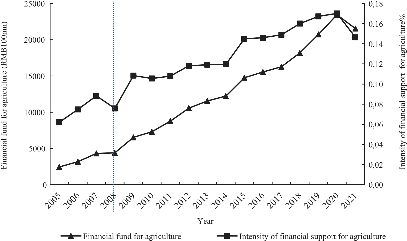
Table 7 reports the regression results of the instrumental variables approach. In Table 7, the Wald test results reached 523.76 and passed the 1% significance level test, indicating that there may indeed be some endogeneity between fiscal expansion and agricultural carbon intensity. The F-value of the first stage regression of the instrumental variable method reaches 195.04, much larger than the empirical value of 10. The coefficient of the instrumental variable is significantly positive, indicating a positive relationship between the instrumental variable and the core explanatory variable fiscal expansion, and there is no weak instrumental variable. Further, in the second stage of regression, after stripping the endogeneity using the instrumental variables, the coefficient of influence of the core variable of fiscal expansion is -0.239. The coefficient of influence of the squared term of fiscal expansion is 0.024, and both pass the 1% significance level test. The results are almost consistent with the coefficient of influence in the base regression, indicating that the model results are robust and reliable.
Table 7.
Estimation results of instrumental variable method.
Conclusions and Policy Implications
Given that the current literature research has not reached a consensus on the relationship between fiscal expansion and agricultural carbon emissions, this paper constructs a theoretical analysis framework of fiscal expansion affecting agricultural carbon emissions based on externality theory and public goods theory and systematically studies the impact of fiscal expansion on agricultural carbon emissions. The findings revealed the following: (1) There is a non-linear U-shaped relationship between fiscal expansion and agricultural carbon intensity, and the fiscal support intensity of agriculture at the turning point is 1.125. (2) The inverse U-shaped relationship between fiscal expansion and agricultural carbon intensity exists only in non-main grain-producing areas and is not significant in main grain-producing areas. (3) Fiscal expansion is conducive to correcting the negative externalities of agricultural carbon emissions, as well as bringing into play the productivity improvement effect and resource allocation effects, which in turn promote the increase of agricultural green total factor productivity and, ultimately, contribute to the reduction of agricultural carbon intensity. This is the primary influence mechanism of fiscal expansion to promote decreasing agricultural carbon intensity. (4) Finally, the decline of agricultural carbon intensity promoted by fiscal expansion is moderated by market segmentation, deviation of industrial structure, and economic growth pressure. (5) Although there may be an inverse U-shaped non-linear relationship between fiscal expansion and total agricultural carbon emissions in terms of impact coefficients, none of them pass the significance test, suggesting that the current evidence is not yet sufficient to support the conclusion that fiscal expansion promotes a decrease in total agricultural carbon emissions after a certain level of fiscal expansion is reached.
Based on the preceding conclusions, this study advances the following recommendations:
Firstly, restructuring fiscal support for agriculture is imperative. Given the generally low agricultural fiscal support intensity across various regions of China, further implementation of moderate and lenient fiscal policies is essential to address the negative externalities associated with agricultural carbon emissions. Optimizing the structure and efficiency of fiscal support for agriculture, delineating clear green and low-carbon subsidy orientations, and integrating fiscal support for agriculture with low-carbon and energy-saving production through precise subsidy mechanisms are vital steps toward enhancing agricultural total factor green productivity and reducing agricultural carbon intensity.
Secondly, bolstering financial assistance for agriculture in major grain-producing areas is necessary. Despite increased fiscal expenditure by the Chinese government in these regions, the level of fiscal support for agriculture needs to be more aligned with their industrial status. Additional efforts should be directed towards concentrating resources and augmenting support for these areas to fully harness the carbon reduction potential of fiscal support for agriculture.
Thirdly, fostering regional collaborative emission reduction is paramount. While state intervention serves as a vital complement to addressing market failures, it must be accompanied by measures to expedite market integration, dismantle barriers to market segmentation, and empower markets to play a pivotal role in resource allocation. Concurrently, leveraging fiscal support for agriculture to drive the optimization and upgrading of industrial structures will fortify the impact of fiscal support on carbon reduction.
Fourthly, integrating agricultural carbon reduction targets into the government’s performance evaluation system is crucial. Embedding agricultural carbon emission reduction metrics into the comprehensive evaluation framework for economic and social development across regions and cadre performance evaluations will facilitate exploring and promoting mechanisms for monitoring and mitigating agricultural carbon emissions. This approach ensures the simultaneous advancement of economic growth and agricultural carbon neutrality.