

Introduction
Data Screening and Preprocessing
Researchers often neglect the screening of data prior to source characterization and apportionment. However, checking the quality of the data can make the interpretation of results easier and more logical. Data screening with/ without pre-processing is essential for several reasons. Since environmental samples are subjected to several steps of processing, including sampling in the field, pretreatment in the lab, chemical or biological analysis, and subsequent modeling, there is a great chance of measurement errors that may spread across several tracers [1, 2]. These measurement errors associated with exposure to air pollutants have negative impacts on the estimation of health effects [3, 4]. Likewise, data acquisition and manual entry into analytical software can lead to errors, because each data matrix involves several variables for each data point [5]. Hence, data preprocessing, particularly data cleansing, is assumed to be an essential step for eliminating such errors. Moreover, owing to the high cost of advanced environmental analysis, the sample size constitutes a challenging issue, and a decision on the balance between the affordability of testing and the attainment of data reliability must be made carefully. In cases of small sample sizes, screening of data to remove errors is an essential prerequisite. Finally, environmental samples are subject to significant heterogeneity, suggesting that data are more sensitive to the existence of data errors [6, 7].
Essential data screening and preprocessing may include, but are not limited to, checking and removing outliers, standardization using the Z scores method, estimation of communalities, checking the existence of multicollinearity, imputation of missing data, and removal of questionable variable/s from the dataset [5, 8]. However, managing environmental quality data differs from managing data in a business and industrial setting, owing to the fact that heavy data cleansing may distort reality, whereas in fact environmental conditions are always changing [1, 9]. Data from environmental observations may not fulfill the condition of normal distribution, particularly data on pollution, which show significant temporal and spatial variability. Fortunately, source apportionment (SA) using receptor models is often applied without data normalization, because the focus is on determining variance rather than means and standard deviation of individual variables. Nevertheless, detections of the aforementioned aspects are all essential tasks for the subsequent interpretation of data and for the robustness and stability of models, in addition to comparability across studies [10].
A brief explanation of these aspects is provided herein, with additional details found in the cited references. Regarding the first aspect of the data screen, the outliers, because all source tracers can be revealed within the context of multiple dimensions, we may assume the existence of multivariate outliers in the data, where each outlier is a combination of unusual values/scores revealed on at least two variables. This could be true with air samples for the purposes of pollution study, where one sample/observation is subjected to analysis of several parameters/tracers; hence, a single observation may reveal several outliers in different tracers, particularly when there is a potential error in lab analysis. Meanwhile, the source tracers/variables can be treated as univariate outliers under the assumption that a single data point is independent of other observations. Being multivariate or univariate, the detection of outliers using quantitative measures can be useful prior to multivariate analysis in both cases [11-13]. The second aspect is multicollinearity, a situation in which two or more variables show a close linear relationship [14, 15]. In reality, multicollinearity exists among the predictors, that is, source tracers, where the same tracer is linked to two or more pollution sources, such as organic carbon (OC) and elemental carbon (EC) from traffic, biomass burning, and coal combustion. The third aspect is estimating communalities, which is an important task for common factor analysis (FA), as the main purpose is to explore the common variance in the data. Communality refers to the proportion of variance in an observed variable that is explained by or attributed to all common (latent) factors in the model [16, 17]. In this study, the observed variables are the source tracers, whereas common “latent” factors are the pollution sources.
On the other hand, data screening or preprocessing for modeling with Unmix and positive matrix factorization (PMF) includes tracing the influence of changing the following aspects: minimum correlation value(R2) for the model run, the number of base runs, uncertainty check with bootstrapping, number of bootstrap runs, change in sample size, and existence of outliers in the dataset [18, 19]. First, since determining the number of sources via Unmix and PMF constitutes a challenge, performing optional Principal Component Analysis (PCA) may be advisable, through which eigenvalues can be obtained directly or estimated from scree plots, which assists in determining the above mentioned number of sources/factors. Second, regarding the estimation of uncertainty, which is a critical step for obtaining relevant and interpretable source profiles, different uncertainties may reflect missing sources, errors in the source profile matrix, and measurement errors. The best way to handle uncertainties is via bootstrapping, which is incorporated into PMF and Unmix [1, 20]. Although source apportionment with software such as PMF.5 provides a useful optional method for evaluating the predictive accuracy and robustness of models via bootstrapping, several researchers ignore this optional step, whereas in Unmix.6, bootstrapping is conducted by default; however, some researchers consider interpreting some output on the uncertainty check negligible [1, 20]. The predictive accuracy and robustness of models using bootstrapping is a validation approach resembling the basic K-fold cross-validation process, in which the original dataset is split into two subsamples: training and test subsamples. Bootstrapping offers unbiased estimates for (internal) validation of model performance. More specifically, in source apportionment, bootstrapping is used to estimate uncertainties in source profiles, which is technically known as robustness, as explained by Norris et al. (2014), although this method has other applications. More details on bootstrapping are provided in the Results and Discussion section of this article. In contrast, one of the drawbacks of bootstrapping is that the number of sources and source profiles identified from bootstrap samples may not necessarily be identical to those of the original dataset, although the newly generated data includes the same number of observations as the original data. Therefore, the investigator needs to map/match the results, that is, matching each factor from bootstrapping with the exact factor obtained from the base run [1, 20, 21]. Third, screening the data for signal-to-noise (S/N) values is suggested to be an important task in modeling with receptor models. Variables with S/N below 0.5 are suggested by Chai et al. (2021) to be excluded, whereas Shiva Nagendra et al. (2021) suggested a threshold value of 0.2, taking into account the importance of the variable, whether it is a typical source signature or a common tracer. Finally, increasing or changing the default number of runs, for instance, gives a chance to look at a better run with the best estimates. Interestingly, with data from a small sample size, increasing the number of runs can be useful given that the investigator has experience in selecting an appropriate number of factors and the ability to identify the potential factors based on the understanding of source tracers [22, 23].
Source Identification and Characterization
Atmospheric pollution sources are conventionally identified and characterized using multivariate methods. In particular, Positive Matrix Factorization (PMF) and Unmix are typical multivariate receptor models of great concern due to several advantages over other models. However, there are critical assumptions applied to receptor models, such as an assumption of mass conservation, non-negativity constraints, normal distribution of errors of the inputs, and the assumption that sources are not correlated in terms of chemical composition. In addition, steady emission profiles to apportion outdoor levels of air pollutants to specific emission sources are the most important assumptions [24, 25]. The negativity constraints, that is, resolving the data to exclude negative values in the analysis, mean obtaining only positive source contributions to the total aerosol mass and positive source compositions, which implies that there is no source involving a negative percentage of a tracer [26, 27]. Both the PMF and Unmix models are based on non-negativity constraints on the composition and contribution of sources [23, 28].
Table 1.
Major source tracers/signatures used for source apportionment
The possible challenges with the application of receptor approaches are the ability to identify the study parameters and the feasibility of obtaining reasonable source profiles that otherwise can result in bias and significant variability across different studies [29]. In practice, conducting source apportionment is a sophisticated process owing to the continuous changes in the chemical properties of pollutants in the atmosphere, and emission characteristics are attributed to multiple sources (as in Table 1), that is, certain tracers are not specific to unique sources. The source tracers/signatures including OC, EC, metals, water-soluble ions, and organic species such as polycyclic aromatic hydrocarbons (PAHs) and some polychlorinated biphenyl (PCBs) are considered major inputs for modeling [25]. Additional challenges include insufficient dispersion parameters included in modeling and overestimation of pollution when winds are parallel to the sources under investigation [24]. It is noted that although the vast majority of studies utilize data obtained from fixed-site monitors, receptor-based approaches can also be used to estimate personal exposure or applied to data from personal exposures [30]. However, receptor models are more affected by spatial variations unless sufficient data from different sampling sites (fixed sites) becomes available [25], unlike emission-based models that have limited capabilities to reflect or resolve temporal variations [31].
Positive Matrix Factorization
The PMF model is a popular multivariate receptor model for the SA of PM2.5 and PM10, based on the assumption of mass conservation of air pollutants. Therefore, conducting mass balance analysis is crucial for identifying and apportioning the sources [29, 32]. Constant source profiles and distinct variations among the contributions are also considered basic requirements for modeling with receptor models such as PMF and Unmix [33]. Interestingly, PMF is suggested as the best choice for source apportionment when limited data on the sources is available, in contrast to chemical mass balance (CMB) models that require prior knowledge of the sources [24]. The PMF v.5, the most recent version upgraded from the PMF.2 program that was initially developed by Paatero (1997), is a multivariate model that utilizes the least-squares method to resolve optimal solutions and estimate the profile and contribution of a source depending on the application of non-negativity constraints, as abovementioned, to promote improved physically reasonable findings [34]. The model assumes P number of sources that contribute to a receptor site. The resolved mass balance equation for the PMF is as follows:
[32]
where Xij is the concentration of species/element j measured in the ith sample, gih is the PM mass level contribution of the hth source to the ith sample, fhj is the mass concentration of species j in (each) source h, and p indicates the total number of independent sources [35, 36]. The estimate ‘e’ is an error between the measured (Xij) and calculated (gih fhj), that is, the residual associated with Xij which has not been accounted for by the factor model. The corresponding matrix form of Equation (1) can be written as follows:
where X is an n×m matrix with n measurements (number of samples) and m elements (the matrix of calculated/ measured data with dimensions of n× m), E is the matrix of residuals with dimensions of n×m, G = n×p matrix of source contributions, and F is a p×m matrix of the source profiles [29]. The object function (Q), which must be reduced as a function of F and G is calculated as follows:
Or
where
where n and m as explained in Equations 1, 2, and 3; Sij the uncertainty of jth chemical species, in samples (ith)[25]
Non-negative constrained weighted values of factor analysis are achieved by minimizing Q with regard to F and G, relying on the restriction/constraint that elements of F and G are completely or partially constrained to nonnegative amounts/values [36]. The uncertainties in modeling with PMF are solved individually for every data point using Equation (6):
Where MDL represents the minimum detection limit of the method and Error is the calculated error of each data value [19].
One of the most important features of modeling with PMF is the FPEAK rotation, a peaking parameter that has no particular scientific theoretical basis for selecting a particular value. Therefore, researchers may apply several FPEAK rotations, with each run using a different FPEAK value (-1.5, -1, -0.5, 0.5, 1). For each run, the researcher checks the values of Q (object function), specifically the lowest Q robust and Q true, which are highlighted by default in PMF.5. Changing the FPEAK values provides a better chance for understanding the rotational freedom of the obtained solutions, with further details about this FPEAK parameter provided in previous studies [37, 38]. In summary, for PMF to solve the task of factor analysis, the program incorporates and resolves all equations from 1–6.
Unmix Model
Unmix is the second-most interesting multivariate receptor model developed by the EPA. A factor analysis method produces only nonnegative/real source profiles and contributions from sources. It has been used fairly in the source apportionment of PM2.5 and PM10 [18, 19, 23, 39, 40]. Interestingly, the simultaneous application of Unmix and PMF generated virtually comparable results regarding the identification of the main sources [41]. However, Unmix can generate solutions that are relatively unstable; that is, source profiles change when the model is run several times [19]. Unmix may produce factors that do not reflect real sources, particularly if the data does not fulfill the model assumptions, and other sources probably share, in space and time, emission characteristics [25]. Similarly, the percentage of source contributions estimated using Unmix may be different from those estimated using other methods [19]. Since the UNMIX model is based on clear mathematical assumptions, its use is highly recommended regardless of the disadvantages, however, it is very important to subject the data to screening prior to UNMIX modeling.
Materials and Methods
Data Screening
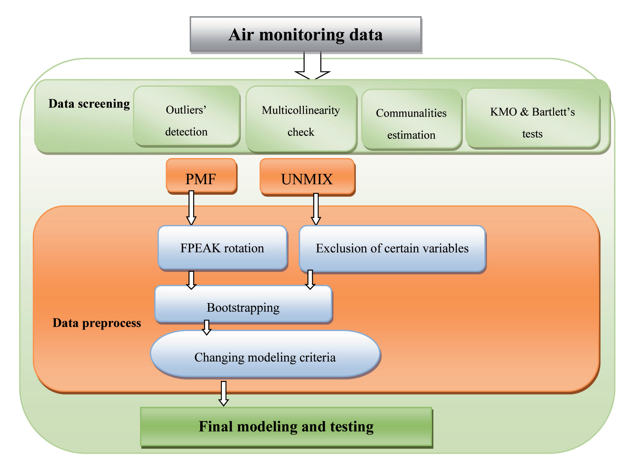
Different data screening tasks are performed, as summarized in the flow diagram (Fig.1). First, we performed a detection of outliers. To detect outliers, we applied Mahalanobis distance, a statistical inference procedure that measures the distance between each data point and the population mean [42]. The Mahalanobis distance is considered a multidimensional generalization for estimating the distance of each point from the population mean, expressed as standard deviation values. Although the approach provides a quantitative result regarding the existence of outliers, it is based on a normal distribution assumption of data, where such an assumption is not always true with real datasets [5, 42].
Secondly, we tested the existence of multicollinearity using the variance inflation factor (VIF) and tolerance statistic values. When VIF exceeds the value of 10, it indicates possible multicollinearity problems, and a similar assumption is applied when the value of the “tolerance” statistic exceeds 0.1 [43]. Thirdly, we estimated the communalities found as an optional step in both PCA and common factor analysis. Initial/prior communalities were estimated using squared multiple correlation (SMC), with values always between 0 and 1. The estimation of communalities is found as an optional step in both common factor analysis and PCA, and we assumed that estimates of communality could be useful prior to modeling with Unmix and PMF, since all are considered factor-based models. After factor analysis, the final measured communalities (extraction) are compared with that of SMC, and if the final communality value is less than that of SMC, it indicates a poor fit or serious problem with the factor model. This implies a need for standardizing the variable, removing possible outliers, or excluding the variable from the analysis. For each variable, “the final communality equals to the sum of the squared loadings.” Meanwhile, although out-of-range communality, also known as Heywood (i.e., values ≥ 1), is expected to result from several reasons, such as insufficient data (i.e. small sample size) and several or fewer common factors, it generally implies that there is a problem with the factor analysis and necessitates further data screening and cleaning [16, 44].
Fig. 1.
Flow diagram of study part1 illustrating the data screening and preprocessing applied in this study
Fourthly, we investigated sampling adequacy by performing the KMO (Kaiser-Meyer-Olkin) test, alongside Bartlett’s test of sphericity, to check the suitability of datasets for factor analysis. These give indications of the suitability of data for receptor models, based on factor analysis and subsequently the reliability of the obtained results [45]. The minimum KMO benchmark value of 0.5, as indicated by Sun et al. (2019), or a value of 0.6, as suggested by Jain et al. (2021), implies the adequacy of the sample size for analysis. In the meantime, when Bartlett’s test of sphericity is significant, it indicates that the study variables are statistically correlated, hence, real factors can be generated [45, 46].
PMF
EPA PMF v.5 software, an upgraded version of PMF2, is capable of performing several mathematical calculations by default or customization [21, 41]. For example, only levels greater than the estimated uncertainties contribute to the signal portion, which eventually contributes to the estimation of S/N ratios. By default, PMF.5 suggests the best-converged solution to be used for further modeling. Meanwhile, researchers may confirm all converged solutions and manually select a reasonable converged solution. The advantage of modeling with PMF.5 is the estimation of uncertainties based on the method detection limit (MDL) values for each individual tracer, as expressed in Equation 7. Additional details on the estimation of uncertainties for below-detection values are provided in various studies [21, 24, 47]. The values of Q (robust) and Q (true) were used to investigate the model goodness of fit, where converged solutions with the lowest Q (robust) were considered for further investigation and modeling [21, 48].
[49]
Initially, the best run for PMF modeling was selected by default when convergence was reached, with the lowest values of Q (robust) and Q (true). More details on the interpretation of Q robust and Q true values are provided in the literature [23, 41, 48]. We observed that increasing the default number of runs led to the selection of a better-converged solution. After the base model, FPeak rotation was performed based on the best run that was initially selected in the base run, and we repeated the attempt to change the number of factors, minimum correlation R-value, and number of bootstraps until a stable solution was obtained. The results of the PMF of major concern are the factor profiles, percentage contributions of tracers to factors, and factor fingerprints. In addition, we investigated the observed and predicted scatter plots to check for possible unusual individual tracer patterns.
Modeling with Unmix
Initially, we included all tracers and the entire dataset (observations) to run the model several times; however, Unmix was unable to produce a converged solution. The model again suggested the exclusion of Ca and Cu tracers, after which only partial solutions were produced. Subsequently, we deleted certain outliers to enhance the stability of the model. This situation implies that additional errors were obtained when all observations were applied, and that reducing the sample size did not affect the stability of the model because the results were comparable to those produced from PMF. This confirms the high sensitivity of Unmix to outliers, missing values, and out-of-range values, such as values below the detection limits. It also suggests that Unmix is more influenced by heteroskedasticity, a situation in which the variance of errors across the observations is not constant, which is often seen in environmental modeling [22]. The initial selection in Unmix utilizes (by default) varimax rotated factor analysis to generate the base model outputs for the species with the highest factor loadings, where Unmix results can further be compared with (optional) varimax rotation results, if necessary.
Sampling and Chemical Analysis
Details of the sample pretreatment and analysis are provided in our previous work [50]. In brief, samples were collected during winter and summer at four receptor sites in Harbin, China, which represent typical residential urban areas, high-traffic roadsides, and low-traffic areas. Particulate matter was collected in quartz filters at a high flow rate of 100 /min. Thereafter, the filters were treated in an oven at 450 °C for 8 h and neutralized in a desiccator at 25 ± 5 °C and RH of 35 ± 5 for 24–48 h. A thermal (optical) carbon analyzer (Model 2001, Desert Research Institute, Atmoslytic Company, United States of America) was used for the analysis of carbonaceous species (elemental carbon and organic carbon) using the IMPROVE-A protocol. Heavy metals were pretreated and analyzed using inductively coupled plasma mass spectrometry (ICP-MS; X series 2; Thermo Fisher Scientific, United States of America). Water-soluble ions were analyzed by ion chromatography (Model Number ICS-90, Thermo Fisher Scientific, United States).
Results and Discussion
Preliminary Results of Data Screening
Regarding the estimation of communalities for each variable, the final communality equals the sum of the squared loadings, as previously mentioned. The values of final communalities are useful in reflecting the existence of potential errors in data and estimating the source percentage contribution of specific sources to individual tracers when interpreted along with other results of factor analysis. From table 2, the final communalities (extraction) of few variables, namely PM2.5 total mass, Na, Ca, Mn, and Cu, were lower than their SMC counterparts. This implies that attention has to be paid while tracing these variables to specific sources, and there may be a need for preprocessing such as normalization or exclusion of outliers. However, since these later variables cannot be deleted, we double-checked the possible errors associated with them by reviewing S/N (Signal-to-Noise) during PMF modeling and the SV (Specific Variance) while performing Unmix modeling, with more details given in the following sections on the findings of receptor models.
Outlier detection is illustrated in Fig. 2, where all values above the UCL (upper control limit) are considered outliers. However, for the data analyzed and included in the main manuscript of this study, outliers were not removed after detection, except for a few outliers removed before Unmix modeling. This was done to examine their effects on the different results of the model and multivariate analysis. To check the influence of sample size on the values of UCL, we arbitrarily split the data into two sets (Fig. 2). In addition, we highlighted the data obtained in summer versus winter to observe the variation in outlier detection. For half of the sample size, although the data showed a low UCL of 5.6, several outliers were detected compared to a high UCL of 20.06. However, quite a few outliers were detected for the entire dataset, suggesting that an increase in sample size minimizes the possible impact of outliers, and this claim has to be interpreted along with the findings of KMO and Bartlett’s tests.
For the multicollinearity check, although several variables showed VIF values exceeding the threshold of 10, the tolerance values were below 0.1, except for Mn, Cu, Na, and Ca, which accounted for overall values of 0.32, 0.22, 0.19, and 0.17, respectively. This implies that checking multicollinearity using more than one measure is useful; that is, relying on one indicator of multicollinearity may be misleading. Modeling with PMF is fairly affected by multicollinearity; therefore, the data must be interpreted with certain precautions if severe multicollinearity is expected [51]. Multicollinearity can lead to instability of the models; therefore, extreme multicollinearity must be avoided [44]. As mentioned by Field (2017), mild multicollinearity has less impact on factor analysis and no effect on PCA, which is one of the reasons why we performed simultaneous PCA and (Factor Analysis) FA analyses in Part II of our study.
Last but not least, the findings of Bartlett’s test of sphericity and the KMO test are shown in Table 4, where the KMO value of 0.833 is far greater than the minimum benchmark KMO score of 0.5, as mentioned in the literature [52]. Therefore, the KMO score indicates the adequacy of the sample size applied for the analysis. Bartlett’s test of sphericity was found statistically significant (χ2 = 3899; df = 276; sig. = 0.001). Hence, the factors generated from modeling are assumed to be reliable and stable.
Findings of Receptor Models
During the initial runs, we performed Bootstrapping to check the predictive accuracy and robustness of models. Interestingly, Bootstrapping requires no specific assumption about the distribution of the original data [1]. Bootstrapping is superior to the basic K-fold method when the original sample size is relatively small. The predictive Accuracy or robustness is measured by bootstrapping across several iterations, in which new bootstrap samples are randomly generated by multiple replacements from the original dataset [53]. In PMF5, the default number of Bootstrap runs, minimal correlation values, and number of seed are all user-defined variables that can be altered based on professional judgment. In contrast, the Unmix model generates Bootstrap samples and runs the model by default until about 100 feasible solutions are produced because it is not assured that feasible solutions will be obtained for each Bootstrap dataset [23]. A feasible solution is characterized by the existence of composition matrices and corresponding contribution matrices for the given set of tracers and observations. We performed matching for each factor from Bootstrapping with the exact factor obtained from the base run or from FPEAK rotation. In the Unmix model, we performed the Bootstrapping for the base run as configured by default, while in PMF5, Bootstrapping was based on the results of Fpeak rotation, i.e. results of Fpeak rotation constitute the basis for carrying out Bootstrapping in PMF. We assumed a source profile is robust if a slight change in model input data results in proportional minor change in outputs [21]. For internal validation, we used parameters such as R2, Bootstrap, etc. for the evaluation [10, 54].
Table 2.
Communalities generated from the factor analysis
Fig. 2.
Multivariate outliers check using Mahalanobis distance for (a) half of the data (59 observations) and (b) entire dataset, with the UCL (upper control limit) set automatically and indicated by dotted line.
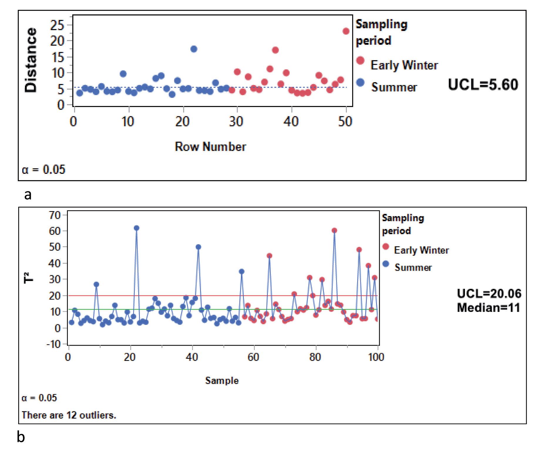
Table 4.
KMO and Bartlett’s test results for the entire dataset
| KMO and Bartlett’s Test | ||
|---|---|---|
| Kaiser-Meyer-Olkin Measure of Sampling Adequacy. | .824 | |
| Bartlett’s Test of Sphericity | Approx. Chi-Square | 3899.194 |
| df | 276 | |
| Sig. | .000 | |
Table 3.
Multicollinearity test
Table 5.
Base run and FPeak run summary
Both PMF.5 and Unmix.6 propose the exclusion of variables from further modeling, though in distinct methods. In PMF, variables/tracers might be removed if their S/N (Signal-to-Noise) values were less than 0.5, as stated by Chai et al. (2021) or less than 0.2, as stated by Shiva Nagendra et al. (2021). Except for Cu and Ca, all variables exhibited a suitable S/N ratio during PMF modeling in this study. In reality, some variables/ tracers are crucial because they are regarded as typical source tracers, and their exclusion may affect the model outputs as a whole. For example, Cl and K (tracers of biomass burning), EC (typical tracers of traffic and coal combustion), and SO4 (tracer of secondary aerosols) are essential tracers [24]. The Unmix model, on the other hand, suggests omitting variables based on an SV (Specific Variance) threshold value of 0.5, above which a variable is indicated for exclusion, while variables with SV values closer to zero are deemed the best for modeling. Occasionally, variables with values somewhat greater than 0.5 SV are kept if they are deemed typical source signatures.
PMF Outputs
In general, the existence of pollution sources that are coincident in time and space constitutes a challenge in multivariate analysis. For instance, the coincidence of vehicle emissions and suspended road dust leads to a perfect correlation between these two sources; hence, their separation becomes difficult. The effects of meteorological conditions on the concentrations of other species that are not considered in receptor modeling [55] and differentiation between diesel and gasoline emissions are all considered challenges of source apportionment [56]. The following are the results of FPeak rotation as part of the PMF modeling, with other outputs summarized in Table 5.
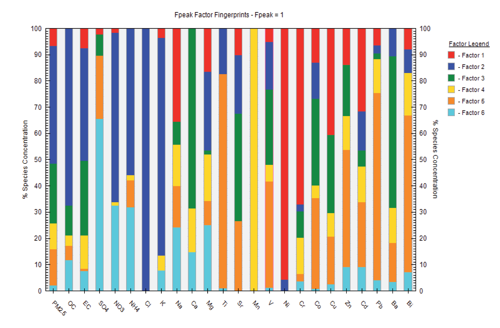
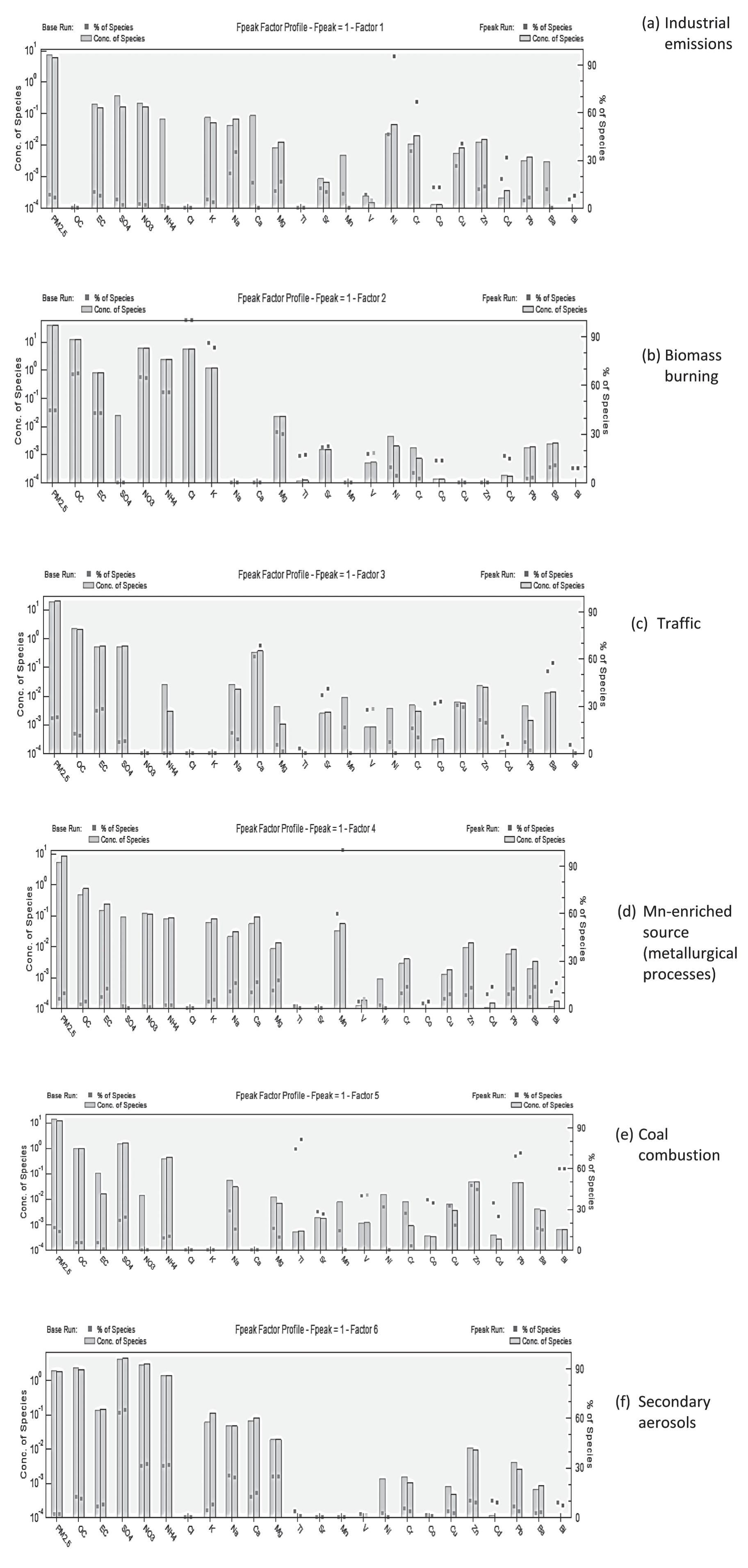
The major sources of air pollutants identified in this study (Figs. 3 and 4) via PMF modeling are biomass burning, coal combustion, traffic, industrial emissions, Mn-enriched sources, and secondary aerosols. Biomass burning as a source of air pollution was identified by typical tracers, such as K and Cl, together with high levels of OC and EC, and moderate levels of NO3 and NH4, in partial agreement with literature [57]. Biomass burning is mainly associated with agricultural activities, the use of wood for domestic heating, and, to a certain extent, the burning of waste. This has a high contribution of approximately 44.7% of PM.5 total mass [46, 58]. The second major contributor to air pollution was found to be coal combustion, contributing to 22.8% of PM2.5 mass and characterized by high levels of Sr, Ba, CO, and EC. Traffic with/without road dust represents the third most dominant source, contributing to approximately 13.8% of urban air pollution, and it is characterized by high loadings of Pb, Ti, Zn, Bi, V, and Ca. This aggregation of Ca with traffic is logical because it may originate from the resuspension of soil and nearby building construction activities. Industrial emissions, which are common sources in most urban areas, and whose contribution varies according to industrialization and economic development in the country, account for 6.8% of total PM2.5 mass concentration [58-60]. Mn-enriched (mainly metallurgical processes) sources contributed to approximately 9.8% of PM2.5 mass. Finally, secondary aerosols (SO4, NO3, and NH4) accounted for an average of 2.1% of source contribution. The contribution of secondary aerosols is greatly affected by weather conditions (photochemical reactions, air temperature, RH, wind); therefore, they show great spatial variability, as explained in literature [23, 61].
The PMF model was more robust and stable compared to Unmix, with respect to changes in sample size and inclusion of variables with missing values; these results resemble those of recent similar studies on the application of PMF and Unmix [18, 62]. The PMF model is also suggested to handle outliers better than Unmix and PCA, which agrees with findings from the literature [23], and source identification using PMF relies on the skills of the researchers, that is, on professional judgment. However, because the PMF model requires no prior knowledge of the nature of the sources under investigation, it is easier for experienced investigators to correctly identify the sources, particularly when it is preceded by data screening.
Unmix Model Outputs
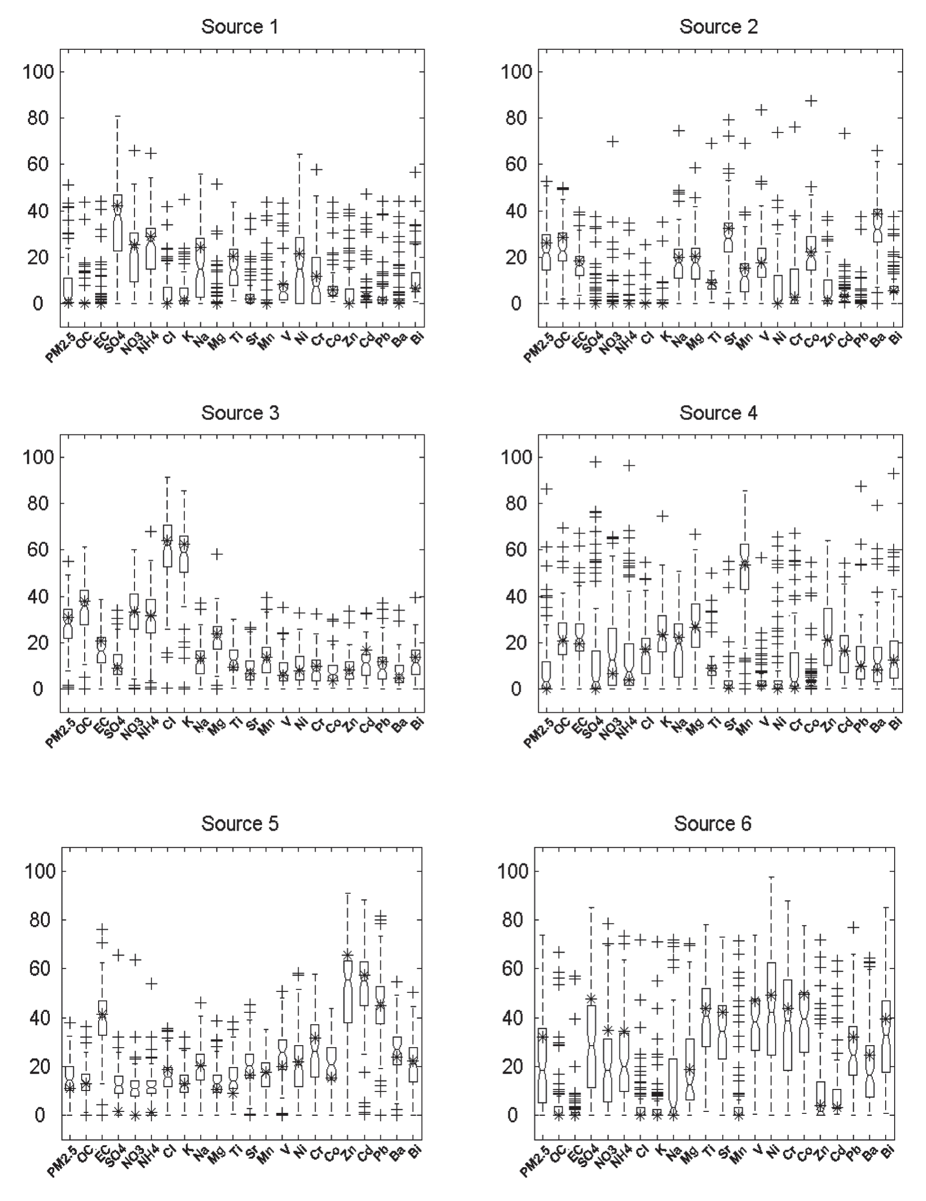
The initial run of the Unmix model suggested the exclusion of Ca and Cu tracers, and it was possible to obtain a converged solution only after this exclusion and the minimization of outliers by eliminating a few observations. Evidently, Unimx is more sensitive than the other methods and requires more data processing, which agrees with the results of Mudge et al. (2017). In terms of the recognition of source profiles and types of sources, both Unmix and PMF recognized similar common sources with comparable profiles, apart from profiles of vehicle exhaust and industrial emissions, which showed slight differences due to possible temporal variability of emissions, in accordance with the literature [22]. However, the estimated percentage variance for each individual source varied between the Unmix and PMF. The mild differences in the percentages of source loadings revealed by PMF and Unmix are acceptable, with no severe effects on the overall results, and are attributed to possible differences in the methods of estimating uncertainties and algorithms [40, 63]. We observed that the solutions predicted by Unmix were relatively unstable where the source profiles were seen to change each time we performed a new run. Unmix was not significantly affected by a slight change in the sample size owing to the removal of outliers, which partially disagrees with the findings of a previous study that indicated the high sensitivity of Unmix to change in sample size [18]. Fig.5 illustrates the source profiles identified by bootstrapping were in brief: source 1 (secondary aerosols); source 2 (coal combustion); source 3 (biomass burning); source 4 (metallurgical process sources with high Mn, and moderate loadings of Zn and Cd); source 5 (traffic); and source 6 (industrial emission sources).
Conclusions
In this study, it was evident that data screening and preprocessing were essential for understanding the nature of the data and gaining insight into the possible impact of errors on modeling outputs. Estimation of communalities and multicollinearity indicated possible data errors in Ca, Cu, Na, and Mn, which affected the stability of source profiles. Further, the effect of outliers decreased with an increase in sample size. We recommend that multicollinearity should be checked using more than one statistical measure, particularly VIF values together with tolerance values. Although data screening is very critical for better interpretation of model outputs, any suggestion for excluding some variables should be considered alongside the reviewing of values of S/N (in the case of PMF) or SV (in the case of Unmix). This is particularly important because a few tracers, such as Cl, K, SO4, and EC, are crucial, and their exclusion could drastically influence the detection of real sources.
PMF has detected major sources, including biomass burning, coal combustion, traffic, industrial emissions, Mn-enriched sources, and secondary aerosols. The Unmix model identified similar sources with comparable profiles, apart from profiles of vehicle exhaust and industrial emissions showing slight differences. Solutions predicted by Unmix were relatively unstable, due to the possible effects of sample size and outliers. Bootstrapping followed by matching each factor from bootstrapping with the exact factor obtained from the base run or from FPEAK rotation is highly recommended because model stability is influenced by errors in data, which is an inevitable problem. PMF was more stable than Unmix, where the latter model was suggested to be sensitive to outliers and Multicollinearity. The simultaneous application of PMF and Unmix, with/without other analytical methods such as FA/PCA and NMDS, could be reasonable for better source characterization and apportionment and for the appropriate estimation of uncertainty.

