

Introduction
The escalating conundrum of global warming, stemming from environmental pollution, stands as a formidable challenge confronting the world. In the pursuit of energy conservation and emission mitigation, numerous countries and governments have instituted policies to govern “carbon constraints”. Of note, freight transportation by road is acknowledged as a primary source of carbon emissions, with the logistics of cold chain vehicles necessitating additional energy consumption to uphold low-temperature environments within their compartments. This, in turn, amplifies carbon emissions. While electric cold chain vehicles offer a viable solution to these challenges, their uptake remains limited owing to inadequacies in charging infrastructure, protracted charging periods, and elevated costs. As the demand for cold chain products surges, logistics companies are increasingly prioritizing distribution efficiency to bolster customer retention rates.
Simultaneously, mounting urban traffic congestion and the concomitant uncertainties that beset road network traffic flows can engender fluctuations in vehicle travel times, thereby influencing delivery schedules, customer contentment, and fuel usage. An ill-suited distribution solution not only begets augmented delivery expenses but also precipitates customer attrition. Presently, several cold chain logistics providers, such as Freshippo and Wedome, have implemented a “reservation system” for pickup and delivery. This necessitates delivery vehicles to effectuate the delivery of cold chain goods within specified time windows, failing which would compromise the quality of the products and trigger corresponding penalties. Hence, there is substantive theoretical and practical merit in investigating the amalgamation of the green vehicle path conundrum, considering carbon emission constraints within a time-dependent network alongside the delivery quandary of cold chain products.
The concept of cold chain logistics was first postulated by Albert Barrier and J.A. Ruddich in 1894. In recent years, within the domain of the Vehicle Routing Problem (VRP), the market scope of cold chain product logistics has exhibited gradual expansion. The optimization objectives of the cold chain product logistics path problem primarily encompass quality assurance, transportation efficiency, and environmental conservation.
Given the temperature sensitivity of cold chain products, it is imperative to reckon with cargo losses within transportation expenses. Scholars have endeavored to address this by quantifying the spoilage of products as a component of transportation costs within their models. Amorim et al. [1] devised a bi-objective optimization model, considering product freshness and distribution costs vis-à-vis the perishability of cold chain products. Meanwhile, Chan et al. [2] incorporated an exponential decay function to lucidly delineate the degradation of product freshness over time, aiming to procure solutions closely aligned with the actual distribution scenario. Gallo et al. [3] formulated a mixed-integer linear programming model to minimize total costs for diverse cold chain products. Afshar-Bakeshloo et al. [4] integrated a segmented linear function to gauge customer satisfaction and developed an optimization model targeting the maximization of customer contentment, minimization of total costs, and curtailment of carbon emissions. Qi et al. [5] delved into the distribution predicament of cold chain products under exigent circumstances, factoring in considerations such as vehicle losses, refrigeration expenditures, and cargo damage costs. They advanced a mathematical model and devised a heuristic algorithm, fusing the Ant Colony System (ACS) with Pareto local search (PLS) to resolve the conundrum. Additionally, Zheng et al. [6] amalgamated multimodal transportation with cold chain logistics, utilizing distribution timeliness and the freshness of cold chain products as proxies for customer satisfaction. They resorted to an enhanced particle swarm algorithm to address the problem.
Scholars generally set the vehicle speed as a constant in advance when studying the VRP problem, and the above problem is called a static vehicle path optimization problem. However, in the actual traffic network environment, under the influence of a variety of uncertainties, the traveling speed of delivery vehicles presents large differences in different time periods, and many scholars have begun to study the vehicle path problem under time-varying road network conditions. Liu et al. [7] propounded a methodology for computing travel times to circumvent traffic congestion in time-varying road networks, with the minimization of total costs as the prime objective. They fashioned an Improved Ant Colony Algorithm and Cultural Algorithm (IACACAA) to effectuate solutions. Franceschetti et al. [8] devised an enhanced Adaptive Large Neighborhood Search (ALNS) algorithm tailored for the time-dependent vehicle routing problem, incorporating novel removal and repair operators to enhance solution quality. Guo et al. [9] modeled the Time-Dependent General Vehicle Routing Problem with Time Windows (TDGVRPTW) in the context of traffic congestion, devising a two-stage hybrid search algorithm to resolve it. Afsher-Nadjafi et al. [10] contended with the heterogeneous vehicle routing problem under time-varying road networks, factoring in constraints such as time windows and vehicle counts, and resorted to heuristic algorithms with the intent of minimizing economic costs. Alinaghian et al. [11] promulgated a novel macroscopic model to calculate fuel consumption in the time-dependent vehicle routing problem, devising an enhanced firefly algorithm to resolve it. Furthermore, Fu et al. [12] delineated a methodology for calculating time-dependent travel times for fresh food e-commerce delivery in the “last mile” conundrum. They aimed to optimize total delivery costs, thereby facilitating open cold chain vehicle product delivery in the context of time-varying road networks. Concurrently, Xu et al. [13] took a comprehensive approach to the vehicle path optimization problem, integrating considerations of time-varying vehicle speeds and customer satisfaction. They devised an integral equation to gauge vehicle fuel consumption and subsequently fashioned the Non-Dominated Sorting Genetic Algorithm II (NSGA-II) to alleviate the problem.
In consonance with the national development tenet of “low carbon and environmental protection,” the reduction of carbon dioxide and associated noxious gas emissions stemming from vehicular operations has emerged as a key research objective. Scholars have endeavored to integrate the abatement of carbon dioxide emissions as a pivotal research goal. Qin et al. [14] introduced a carbon trading mechanism to calculate the cost of carbon emissions and analyzed the impact of carbon prices on total costs, carbon emissions, and average customer satisfaction. Zulvia et al. [15] constructed the Carbon-Efficient General Vehicle Routing Problem with Time Windows (GCVRPTW) to encapsulate the carbon dioxide emissions attributed to cold chain products and their implications on distribution costs. Küçükoglu et al. [16] devised an adaptive simulated annealing algorithm to resolve the cold chain logistics problem, with the aim of curbing travel distances, penalty costs, fuel consumption, and carbon emissions, given the high energy consumption. In a similar vein, Li et al. [17] introduced a novel fuel and carbon emission model within the context of the heterogeneous vehicle path problem, accounting for vehicle carbon emission costs in light of fuel consumption. They resorted to an improved forbidden search algorithm to resolve the problem. Chen et al. [18] explored the cold chain path optimization problem with forward storage from a low-carbon perspective, transforming carbon emissions into one of the objectives, and proposed a hybrid simulated annealing tempering algorithm to solve the problem.
In summary, scholars’ research objectives for cold chain logistics can be categorized into three areas: quality assurance, road transportation, and environmental protection. Based on this, this paper takes the logistics and distribution of cold chain products as the main body of research, designs the quality change function to express the special characteristics of cold chain products, designs the time-varying speed of vehicles to avoid traffic congestion, takes the minimization of the comprehensive cost as the objective function, considers the constraints such as regional and district carbon emission management, vehicle loading, and soft time window of customers, and by fusing the genetic algorithm and the large-scale neighborhood algorithm, a hybrid algorithm is designed to solve the problem, which aims at realizing the realistic road network for the distribution of cold chain products under the constraints of carbon emission.
Problem Description and Method Design
Problem Description
A cold chain logistics enterprise performs cold chain product distribution tasks for N customers, the geographic location, demand, and time window of each customer point are known, and the demand of each customer is less than the capacity constraints of the vehicle. Considering the various costs of cold chain logistics and distribution comprehensively, the aim is to seek the path that minimizes the total cost of vehicle operation under the premise of satisfying constraints such as the rated vehicle loading and the soft time window of the customer.
To elucidate the applicability of this study, the following assumptions are posited:
(1) There is only one distribution center, and its location is always fixed.
(2) The vehicles dispatched from the distribution center are uniform in nature.
(3) The cold chain products transported belong to the same category and necessitate identical cold storage conditions.
(4) Vehicle speed variations are only affected by the time period in which they occur and do not take into account other incidental and sudden factors.
(5) The perishability of fresh products is solely contingent on time, with the exclusion of other incidental factors such as inadvertent human error.
(6) The distribution area has the same carbon constraint capacity.
Calculation Method for a Time-Dependent Vehicle Travel Time
In the real road detection system, the degree of road congestion will be updated every once in a while, so this paper simulates the same scenario, assuming that the vehicles are traveling at different speeds in different time periods. Based on the “first-in-first-out” criterion, divide the working time of the logistics centre into a set of S time periods of length Z,
Let
Step 1: Vehicle travel time calculation for the departure time period.
Step 2: Vehicle travel time calculation for subsequent time segments. (1)
Model Build
Symbols and Variables
Symbols: N is the set of customer points, N = 0 denotes the distribution center, K is the set and sum of cold chain vehicles provided by the distribution center; and Qm is the maximum load capacity of the vehicle, qi is the demand at customer point i,
Variables:
Logistic Cost Analysis
(1) fixed costs
Fixed costs of vehicles, the acquisition costs of vehicles, routine maintenance costs, and driver salaries are related to the number of logistics vehicles used, and the fixed costs of vehicle use are:
(2) Fuel costs
In the process of vehicle transportation, the fuel consumption of vehicles comes from two parts: one part is the fuel consumption generated by the engine of the transportation vehicle during transportation, and the other part is the additional fuel consumption due to the use of refrigeration equipment.
(ⅰ) Fuel costs incurred by transportation
The fuel consumption of the distribution vehicle is calculated with reference to the CMEM model proposed by Barth et al. Disregarding the effect of road gradient and acceleration on the fuel consumption of the vehicle, the vehicle moves from point i to point j to perform the distribution task, assuming that its traveling time is
Where
(ⅱ) Fuel costs incurred by refrigeration
Cold chain logistics vehicles will be subjected to thermal loads on the way of distribution, and the role of refrigerant is to inhibit the temperature changes brought by thermal loads. The heat load mainly consists of two parts: one is the heat transferred from outside the compartment to inside the compartment, i.e.
The fuel cost C2 incurred throughout the distribution process can be expressed as:
(3) Penalty costs
In the process of logistics and distribution, customers have certain requirements for time. Assuming that the time window in which the customer expects to be served is
The time punishment cost C4 of the entire delivery process can be represented as:
(4) Cargo damage costs
Cold chain products are easily affected by factors such as temperature, humidity, and the oxygen content of the air, and cause a certain degree of loss. When the loss reaches a threshold, it will cause corresponding damage to the goods. For product damage, the introduction of quality corruption functions
Based on the above analysis, the mathematical model is developed as follows:
Where the objective function (10) denotes the total cost of distribution. Constraint (11) denotes the rated load of the vehicle; constraint (12) denotes the total carbon emission constraint of the vehicle; constraint (13) denotes that the demand of each customer point can only be satisfied by one vehicle in a single trip; constraint (14) denotes that each vehicle arrives and departs at the same customer point; constraint (15) denotes that each vehicle departs from and returns to the distribution center; constraint (16) denotes the continuity of distribution time; constraint (17) denotes the relationship between roadway distance and the distance traveled in each time period; and constraint (18) denotes the decision variables.
Algorithm Design
The VRP belongs to the NP-hard problem, and the CVRPTW under the time-varying road network is considered to be more cumbersome, and how to solve it accurately and efficiently is a major challenge. In existing research for solving similar problems, heuristic algorithms are often used, and the genetic algorithm among the heuristic algorithms has been widely developed and applied because of its stronger robustness, higher practicality, and more mature theory. Therefore, this paper improves the genetic algorithm, combines the genetic algorithm with a large-scale neighborhood search algorithm, and designs a hybrid genetic algorithm.
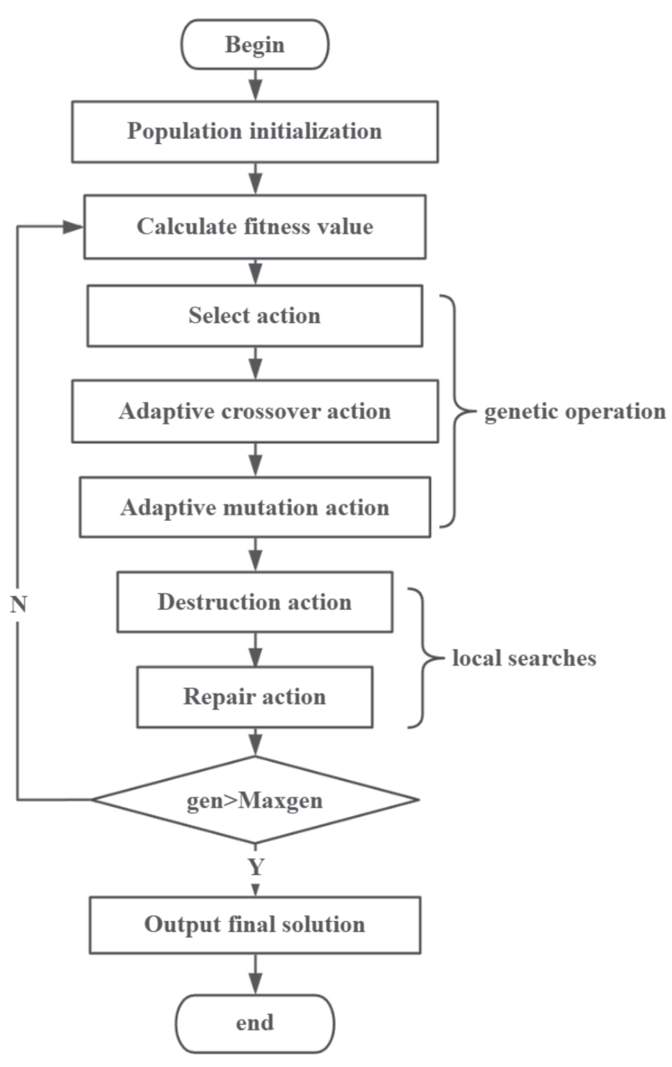
Compared with the traditional genetic algorithm, the hybrid genetic algorithm improves the optimization ability through large-scale neighborhood search, and the improved cross-variance operator continuously optimizes the feasible solution. At the same time, the optimal individual continues to be unchanged for a number of generations as the basis for the judgment of the stopping of the iteration, which avoids a large number of ineffective redundancies of iterations, thus improving the solution efficiency. Compared with traditional neighborhood search, the algorithm not only maintains the optimal search capability of large-scale neighborhoods but also overcomes the weakness of inefficiency, thus improving the quality of local optimal solutions. However, the algorithm’s optimization process takes some time due to the relatively long iteration time. In the early optimization stage, the algorithm mainly relies on the global search capability of the genetic algorithm and the local search capability of the large neighborhood algorithm to rapidly approach the global optimal solution through improved crossover and mutation operations, while in the late optimization stage, it mainly relies on the local search capability of the large-scale neighborhood search algorithm to help the algorithm jump out of the local optimal solution by destroying and reconstructing the current optimal solution through the remove-insert operation. This combination effectively balances the algorithm’s local optimization ability and global optimization ability and improves the algorithm’s solution performance. The flow of the algorithm is shown in Fig. 1.
Encoding and Generating Initial Solutions
Real number encoding of the chromosome. A chromosome is randomly generated, and the initial population is obtained by decoding the individual customer points in order and dividing them into vehicles based on their load constraints and the moment of return delivery time.
Fitness Function
This paper is an objective function minimization problem, so the choice of the fitness function is measured by the inverse of the objective function as follows:
In the above equation,
Select Action
Aiming at the disadvantageous problem that the roulette method needs to repeat the selection N times, random traversal sampling is proposed as another selection method, and its main direction of improvement is that it only needs to generate N equally spaced marking pointer positions at a single time to get the population containing N individuals, and in this paper, we mainly use random traversal sampling method to complete the selection operation.
Crossover and Mutation Action
In genetic algorithms, setting a fixed crossover probability and mutation probability can guarantee the production of new individuals, but when the population evolves to a certain degree, it is easy to destroy the individuals with higher adaptation. So this paper introduces the improvement method of adaptive adjustment and sets the crossover probability for individuals as follows:
Where
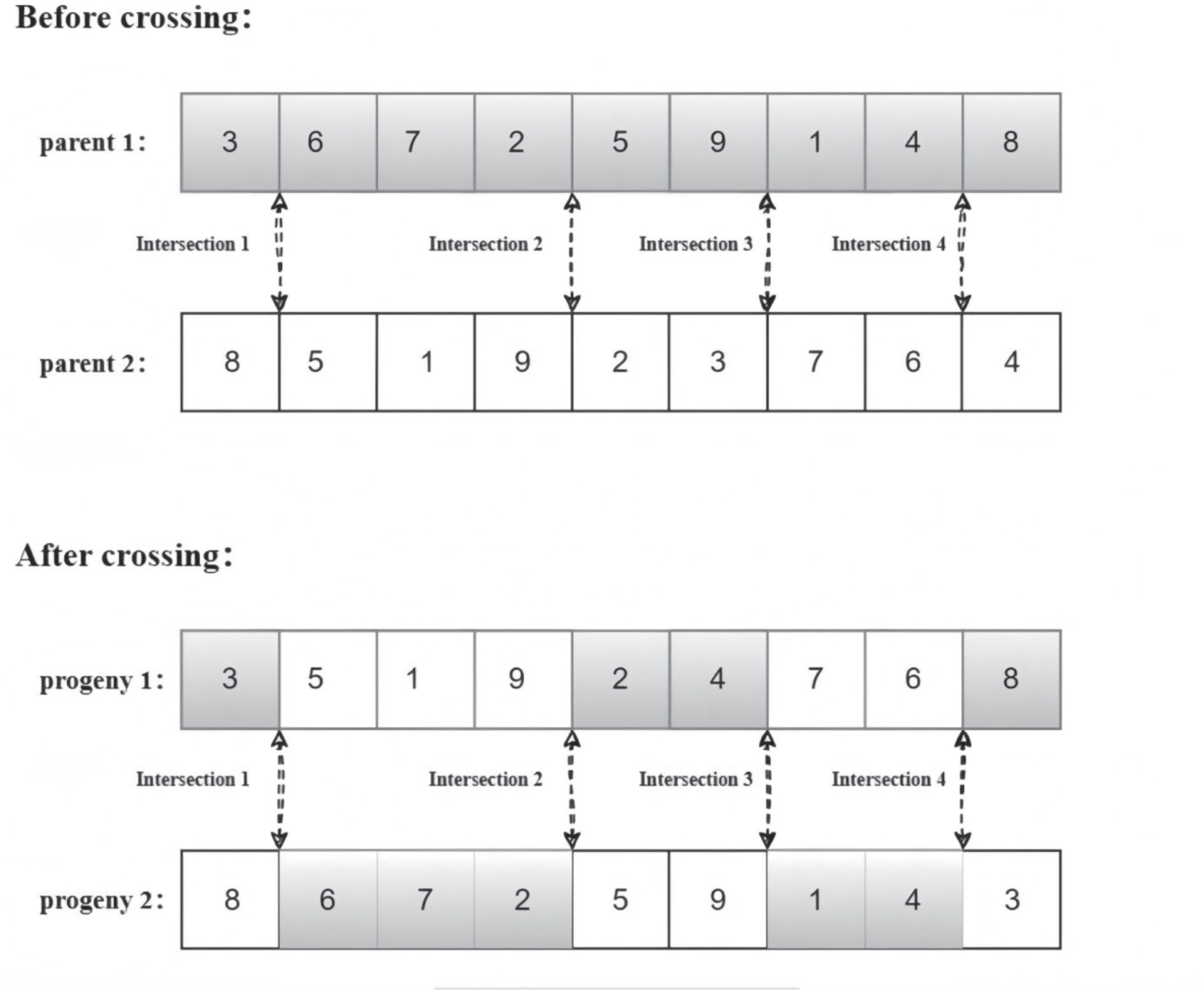
For any chromosome Pi , if Pi < Pc , then chromosome xi goes to the crossover operation, and vice versa for the next generation, the crossover method used in this paper is shown in Fig. 2.
In the same way, in order to ensure the continuity of the best individuals in the population, this paper sets the dynamic probability of mutation, which is set as follows:
Where
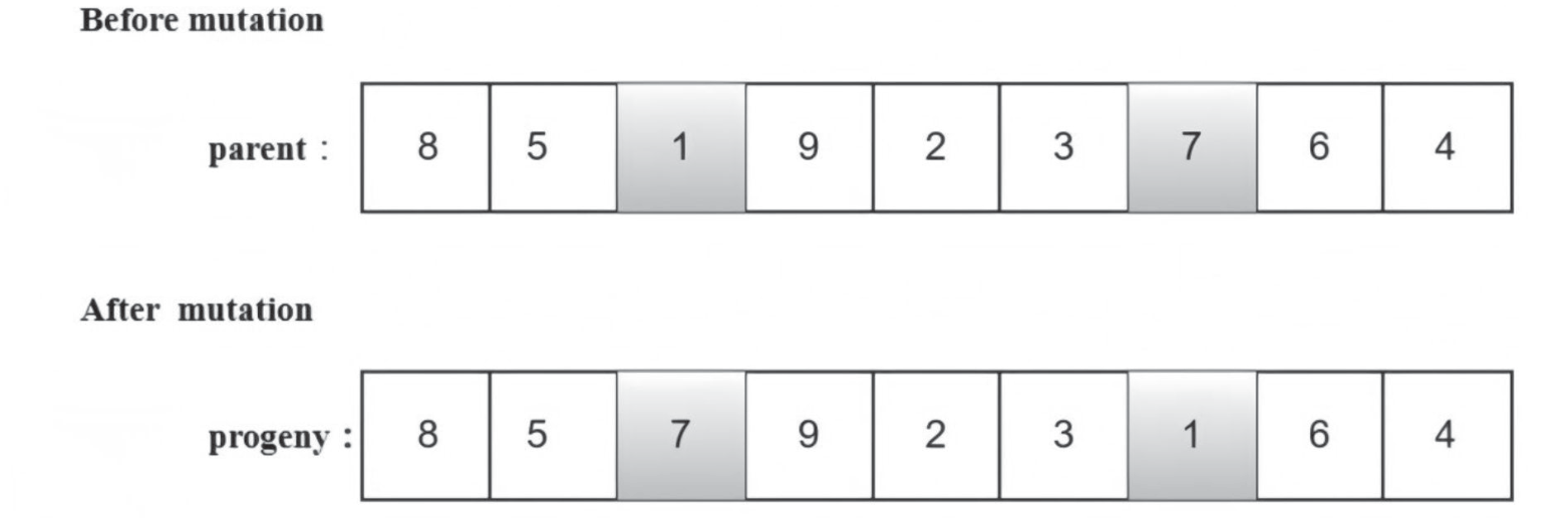
For any chromosome Pi , if Pi < Pm , the chromosome xi enters the mutation operation, and vice versa, it enters the next generation, the mutation method used in this paper is shown in Fig 3.
Local Searches
In order to optimize the results of the genetic algorithm, this paper adopts a large-scale neighborhood search algorithm for local search operations, which is mainly accomplished through two links of constant “destruction” and “repair”.
Destruction operation: σ denotes the current solution, c denotes the client points to be removed, C denotes the set of removed client points,
Where,
To verify the validity of customer point removal, a stochastic element is introduced, whereby customer points are randomly selected from a correlation sequence ordered from highest to lowest.
Repair operation: according to the vehicle load and time window constraints, to find the best insertion position of each customer point in the set C in σ', the best insertion position is inserted after the vehicle distance is increased by the smallest position. Then calculate the target increase value of each customer point in C after inserting it into the best position, select the customer point with the largest target increase value as the first inserted point, and repeat this operation until all elements in set C are inserted into σ'.
Experimental Design and Analysis of Results
Design of Experiments
(1) Parametric design
The algorithm is programmed using the software Matlab R2023b for algorithm programming with a CPU of 3.40 GHz, an operating system of Windows 10, and a computer with 8GB of memory.
The parametrics of the algorithm are set to
In the calculation of the vehicle fuel consumption and carbon emissions,
(2) Calculation of Instances
Take a cold chain logistics company as an example. The distribution center needs to complete the distribution service of cold chain products to 20 customer points on the same day. The coordinates of the distribution center are (35,35), the vehicles of the distribution center depart from the distribution center at 6:00, and the maximum load capacity of the cold chain vehicles is 9t. The data on the demand of each customer point, the allowable time window, the desired time window, and the service duration are shown in Table 1, and the example data are from the literature [19].
Calculations show that three vehicles are needed to accomplish this distribution task at a cost of ¥3037.2625, and the path of each vehicle is as follows:
(1) Vehicle1:0-13-8-14-12-7-0;
(2) Vehicle2:0-20-1-2-19-6-17-18-16-15-0;
(3) Vehicle3:0-5-4-3-9-11-10-0.
(3) Calculation of Examples
In order to further verify the applicability of the algorithm, the coordinates, demand, time window, and service duration of different distribution types (C distribution, R distribution, and RC distribution) in Solomon’s VRPTW algorithm are selected as the basic data for testing in this paper. Meanwhile, for the problem of hard time window in Solomon data, in order to better match the real logistics and distribution situation and set the soft time window of the customer, the following modification is made to the Solomon data: the time window of the customer in the data is taken as the desired time window, and on the basis of the desired time window, the time window on the left side is -20 (to ensure that the value is non-negative), and the time window on the right is +25, and the generated time window is taken as the allowed time window of the customer.
(ⅰ) Small-scale example
The example R105 (1*20) in Solomon’s data is chosen for solving the problem, the location coordinates of the distribution center are (35,35) and the working time window [0,230], and the distribution scheme is obtained as shown in Table 2, where D stands for the distance traveled (km), T stands for the time traveled (hours), and C stands for the total cost of the distribution scheme (yuan).
(ⅰⅰ) Medium scale example
The example RC208 (1*50) in Solomon’s data is selected for solving, the location coordinates of the distribution center are (40,50), the working time window is [0,960], and the distribution scheme is obtained as shown in Table 3.
(ⅰⅰⅰ) Large Scale Example
The example C101 (1*100) in Solomon’s data is selected for solving, the location coordinates of the distribution center are (40,50), the working time window is [0,1236], and the distribution scheme is obtained as shown in Table 4.
Table 1.
Example data.
Analysis of Results
(1) Algorithm analysis
To further verify the superiority of the AGALNS algorithm. Comparative analysis of the algorithms is carried out on nine sets of Solomon arithmetic cases with different distributions, and the computational results of the traditional genetic algorithm (GA), large-scale neighborhood search algorithm (LNS), and AGALNS in this paper are given in Table 5. Each algorithm is run 10 times to get the optimal result. Where TC denotes the total cost, VD denotes the total distance traveled by the vehicle (in kilometers), VT denotes the total time traveled by the vehicle (in hours), and IR refers to the saving ratio (%) between AGALNS and the total distribution cost of GA and AGA.
From the results in Table 5 it can be seen that:
1) according to the value of TC, the total cost of AGALNS is better than the values obtained by GA and AGA in all the cases, with the lowest saving of 0.03% and the highest saving of 6.95%, which indicates that AGALNS can effectively reduce the cost of logistics and distribution; 2) as shown by the values of VD and VT, the distance and vehicle traveling time of AGALNS are better than those of the values obtained by GA and AGA in most cases, especially the advantages are more obvious in the data sets of type R (random distribution) and type RC (mixed distribution), which is due to the fact that the customer set is more concentrated than type C (concentrated distribution). time are better than the values obtained by GA and AGA, especially in the data sets of R (random distribution) and RC (mixed distribution). This is due to the fact that the customer set is more diffuse than C (centralized distribution), which makes it easier to plan the optimal vehicle paths according to the time-varying road network, and also shows the applicability of the AGALNS algorithm on real roads.
Table 3.
Medium-example vehicle path optimization results.
Table 4.
Large-scale calculation of vehicle path optimization results.
(2) Sensitivity analysis
(ⅰ) Comparison with a vehicle traveling at a constant speed
In order to verify the effect of vehicle speed on the vehicle path results, the time-varying road network is compared and analyzed with different constant speed schemes, and Table 6 shows the optimal results for ten runs. Among them, Case1 represents the speed under a time-varying road network, Case2 represents the constant speed of 35 km/h, Case3 represents the constant speed of 45 km/h, Case4 represents the constant speed of 60 km/h, Case5 represents the constant speed of 75 km/h, N represents the size of the customer, TC represents the optimal solution of the results of the ten runs, GAP is the optimal solution of the results of the 10 runs of the vehicle traveling at a constant speed, and the optimal solution of the results of the 10 runs of the vehicle traveling at a constant speed is obtained with the speed-time dependence. GAP is the relative error between the optimal solution in the calculation results and the optimal solution obtained when the vehicle speed is time-dependent.
As seen in Table 6, the optimal solution for the same customer size changes with the speed; the faster the vehicle speed, the smaller the travel time, the smaller the penalty cost incurred, and the smaller the optimal solution. This underscores the significance of factoring in vehicle speed when devising distribution strategies.
(ⅰⅰ) Analysis of different carbon constraints
To examine the impact of carbon restriction magnitude on vehicular route outcomes, three experimental sets featuring distinct carbon constraints are formulated and resolved across varying customer volumes. Table 7 presents the optimal outcomes of ten iterations. Here, Case1 denotes CO_Max = 1000, Case2 represents CO_Max=800, and Case3 signifies CO_Max=600, with N indicating customer volume, and GAP representing the relative discrepancy in optimal solutions under distinct carbon constraints as compared to the CO_Max=1000 optimal solution.
As can be seen from Table 7, the optimal solution increases with the carbon constraint for the same customer size, i.e., the stronger the constraint on regional carbon emissions, the larger the corresponding incurred cost, which is due to the increase in the penalty cost due to the violation of the carbon constraint. The comprehensive scrutiny of arithmetic examples across various scales underscores the imperativeness of incorporating carbon constraints in urban cold chain transportation.
Table 5.
AGALNS Comparing the algorithm with the GA algorithm and the AGA algorithm.
Table 6.
Comparison between time-varying road network and constant speed state.
Conclusions
The inefficient distribution of fresh products has always been a close concern for cold chain companies, and it is of great practical significance to take into account the environmental protection and distribution efficiency of cold chain enterprises. In this paper, in view of the reality of today’s urban road congestion, carbon emission restrictions in urban areas, and low distribution efficiency, we design the vehicle travel time calculation method and cold chain product quality function under time-varying road network, and then we establish TDGVRPTW by taking the constraints of the fixed carbon emission, vehicle loading, and the customer soft time window and taking the customer’s timeliness requirements for express parcels and the expectation of the logistics company for cost optimization as the objectives. model and solve it with the AGALNA algorithm. The research has accomplished the following:
(1) Referring to the existing literature, solving the example of a cold chain company to get the logistics and distribution scheme, and at the same time, selecting several sets of Solomon’s arithmetic cases for solving and analysis, verifying the applicability and generalization ability of the algorithm; (2) Solving the VRPTW of the same scale by the standard genetic algorithm and adaptive genetic algorithm, verifying that AGALNS has a better solving quality; (3) The TDGVRPTW model and the GVRPTW model are used to solve on the same scale size of Solomon’s arithmetic case, and it is found that the TDGVRPTW model is able to better avoid traffic congestion and improve the distribution efficiency; (4) Aiming at the environmental carbon emission limitation, different carbon constraint strengths are set in the same scale size of Solomon arithmetic case, which proves that the carbon constraint capacity is closely related to vehicle path planning and effectively promotes the harmonious development of fresh food distribution and environmental protection.
Future research will consider factors such as multiple vehicle types, variable customer demand, variable traffic capacity, and variable delivery addresses to bring the problem closer to reality and to improve and develop more efficient solution algorithms.