Introduction
Historically, to guarantee the feeding of the world population, agriculture has been the activity that has consumed the greatest amount of water [1]. Approximately 40% of the world’s food depends on activities inherent to agricultural irrigation [2]. This constantly increasing water demand [3] can trigger significant meteorological droughts [4–6], which are accentuated in arid regions [6, 7], where the incident solar radiation (SR) is more intense [8, 9]. Intense SR causes approximately 60% of precipitation to return to the atmosphere in the form of evapotranspiration [10, 11], causing these regions to be classified as vulnerable to desertification [12]. For example, in semi-arid regions, agricultural irrigation is a parameter that should trend toward intelligent irrigation [13–16]. To develop intelligent irrigation, valuable information must be available that establishes the relationship between crop growth and water balance [17], in which reference evapotranspiration (ETo) is essential [18]. According to [19] and [20], ETo is the potential evapotranspiration of a hypothetical grass surface with uniform height, well-watered, and active growth, and which depends entirely on climatological variables [9, 21]. According to [9, 22–24], it is always advisable to use empirical equations to estimate ETo by the Penman–Monteith (PMC) method, even when data is lacking, mainly because it remains the most precise method. Of alternative methods, Hargreaves (HAC) continues to be the most used, mainly due to its high accuracy/number of variables used ratio [25–27]. However, [26, 27] state that another possible way to estimate ETo by Penman–Monteith is through simple linear regressions (SLR) and simple nonlinear regressions (SNR); PMR (dependent variable) vs HAC (independent variable), which more accurately calculates the hydric requirements of crops.
In Mexico, approximately 77% of the volume of the total water resource is allocated to the agricultural sector, and two-thirds of the national territory is characterized by an aridity index ranging from arid to semi-arid [13]. In particular, the state of Sinaloa has a predominantly semi-arid climate [7], and according to [13, 23], this condition predisposes it to focus efforts on the characterization of PMR, as well as the subsequent design and administration of intelligent irrigation systems [13, 23]. Intelligent irrigation could improve the volumes of yields of Sinaloan crops as well as encourage the conservation of water resources [23, 28].
In this study, daily series (1979–2017) of minimum (Tmin) and maximum (Tmax) temperatures were obtained from seven weather stations in Sinaloa from the National Water Commission (CONAGUA) [29]. PMC, HAC, and PMR were calculated. At another weather station, Acaponeta, observed daily series (2005–2008, 2011–2013, and 2015– 2017) were obtained of mean temperature (Tmno), incident solar radiation (SRg), average relative humidity (), and average wind speed at a height of 10 m (). The data for the eight stations were provided by the CONAGUA [29] and CONAGUA–National Meteorological Service (SMN) (CONAGUA–SMN) [30]. At Acaponeta, daily observed Penman–Monteith ETo (PMO) was calculated. For validation, three SLRs were obtained: SR vs SRg, PMC vs PMO, and PMR vs PMO. A hypothesis test was applied: Pearson correlation (Pr) vs Pearson critical correlation (Pcr). In the three SLRs, the condition Pr > |Pcr| was met; that is, all Pr were significantly different from zero [31].
The goal was to create PMR estimation models using latitude–temperature data for the state of Sinaloa, Mexico.
Although most of the weather stations for public use in Sinaloa lack the full set of climate variables necessary for the calculation of PMO [7], in this study, predictive models of PMR are provided using the variables latitude–temperature. These models can help ensure the feeding of “the breadbasket of Mexico” through intelligent irrigation [13, 23].
Materials and Methods
Study Area
Sinaloa is in the northwest of Mexico (Fig. 1), and because it is the most important agricultural state in Mexico, it is called “the breadbasket of Mexico” [32]. Furthermore, this state is the main producer of export-oriented crops [33] cited by [32]. Due to the planted area and sensitivity to extremes of RHO–Tmax–Tmin, two of the most important crops in Sinaloa are corn and beans [28].
Data
Daily Maximum (Tmax) and Minimum Temperature (Tmin)
Using data from CONAGUA (https://smn.conagua. gob.mx/es/climatologia/informacion-climatologica/ informacion-estadistica-climatologica) [29], daily series of Tmax and Tmin were obtained from 70 weather stations in Sinaloa for the period 1942–2019. These same series were previously obtained by [34]. Through a review of the availability of recent information (< 5% missing data), in this study, it was decided to work with seven weather stations (Culiacán, El Playón, Las Tortugas, Rosario, La Concha, Ixpalino, and Sanalona II) for the period 1979–2017 (Fig. 1).
Imputation of Missing Data, Homogenization of Series, and Determination of the Mean Daily Temperature (Tmn)
Using RStudio software, with the Climatol library [35] and the orthogonal regression method, missing daily data of Tmax and Tmin were estimated by imputation. Using the standard normal homogeneity test (SNHT) [36] method, with Climatol, the series was also homogenized. By means of the semi-sum of the complete and homogeneous series of Tmax and Tmin, the daily series of Tmn was determined.
In general, the greatest thermal extremes were registered in Ixpalino (Tmax = 46.50°C day−1), El Playón and Las Tortugas (Tmin = −6.00°C day−1), and El Playón (Tmn = 38.00°C day−1, Table 1).
Wind Speed at 10 m Height (Uz)
Through the National Oceanic and Atmospheric Administration (NOAA) [37] (https://downloads.psl.noaa. gov/Datasets/ncep.reanalysis2/Monthlies/gaussian_grid/), the monthly series (Jan–Dec) of wind speed at a height of 10 m (Uz) were obtained for the period 1979–2017. Due to the availability of satellite information, Uz was obtained for only two coordinates in the state of Sinaloa: 1) 25°43′14″ N by 108°45′00″ W and 2) 23°55′42″ N by 106°46′48″ W.
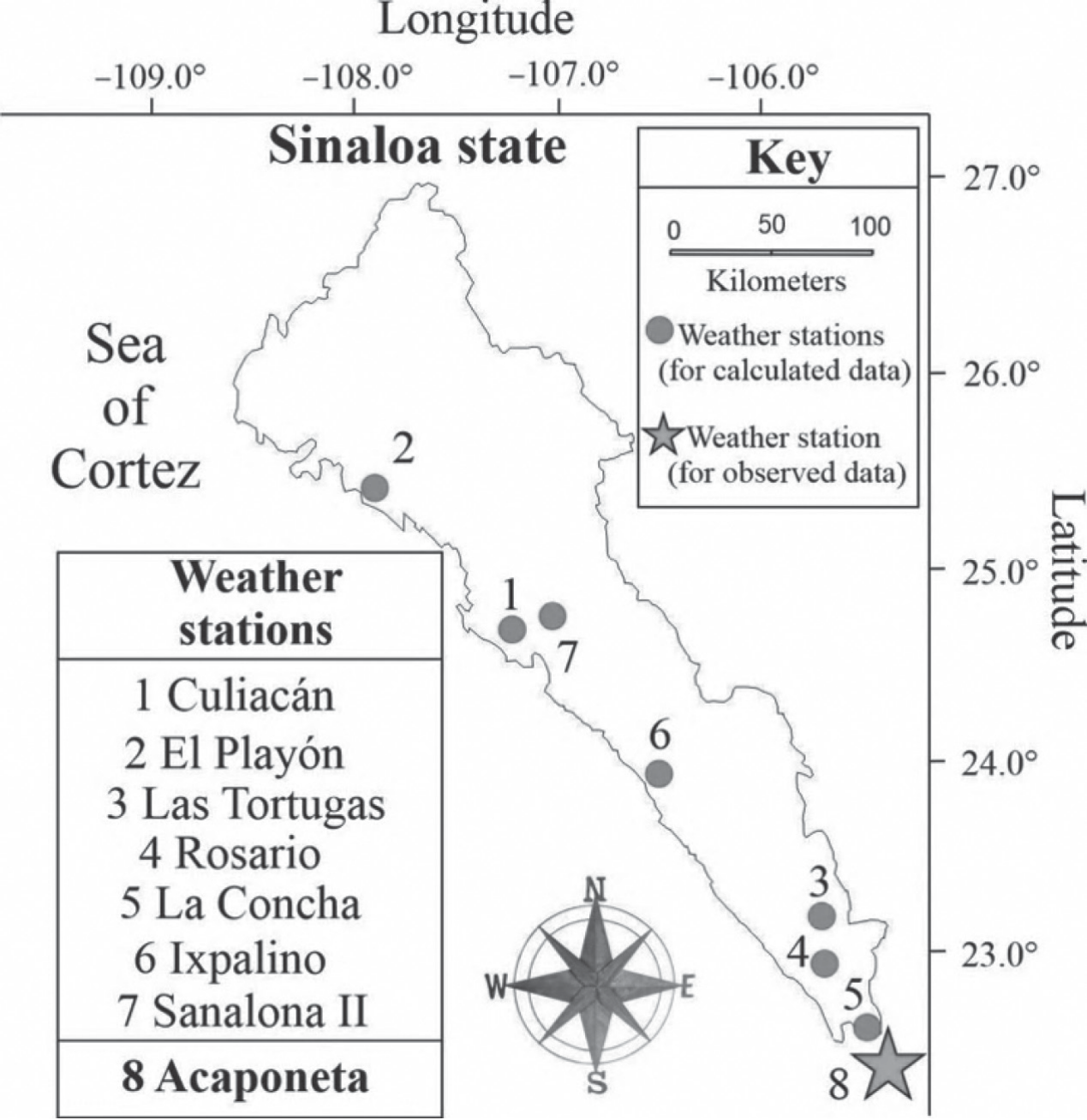
Table 1.
Maximum, minimum, and average values of the maximum (Tmax), minimum (Tmin) and mean (Tmn) temperatures, in Sinaloa, for the period 1979–2017.
Empirical Equations to Estimate Penman–Monteith Reference Evapotranspiration, Calculated with
Missing Data (PMC̄) and Observed Data (PMO)
Wind Speed at 2 m Height (U2)
Although [9, 38] states that wind speed is not very relevant for estimating PMC in semi-arid regions, in this study, using Equation 1, the wind speed was obtained at a height of 2 m (U2) [19, 22].
where U2 = monthly average wind speed at a height of 2 m (m s–1), Uz = average wind speed measured at a height of 10 m (m s–1), and z = measurement height of Uz (m).
Since PMC is the international standard because of its greater measurement accuracy [9], in this study, PMC was estimated daily using Equations 2–10. These equations, which are recommended by [19, 22] when there are missing data, are given as follows:
where eaC = calculated actual vapor pressure and Tmin = daily minimum air temperature (°C).
where es = saturation vapor pressure (kPa) and Tmn = daily mean air temperature (°C).
where ∆ = slope of the saturated vapor pressure curve (kPa °C–1).
where SR = calculated incident solar radiation (MJ m–2 day–1), KRS = solar radiation adjustment coefficient (dimensionless), with a value of 0.16 for continental conditions and 0.19 for coastal conditions (in this study, KRS = 0.16 was used), Tmax = maximum daily air temperature (°C), and Ra = extraterrestrial solar radiation (obtained through tabulated values with respect to latitude, MJ m–2 day–1).
where SRo = incident solar radiation with clear sky (MJ m–2 day–1).
where Rnl = net longwave radiation (MJ m–2 day–1), σ = Stefan–Boltzmann constant (0.4903×10⁻⁸ MJ K–4 m–2 day–1) and TmnK = mean daily air temperature (°K4).
where Rns = net shortwave radiation (MJ m–2 day–1).
where Rn = net radiation (MJ m–2 day–1).
where PMC = Penman–Monteith reference grass evapotranspiration (mm day–1, calculated with missing data), PMO = Penman–Monteith observed grass reference evapotranspiration (mm day–1, at the Acaponeta station), G = soil heat flux density (MJ m–2 day–1, null for daily estimates), and γ = psychrometric constant (0.067 kPa°C–1; tabulated value by [19, 22], for stations with altitudes ranging from 0 to 100 masl).
Calculated Hargreaves Reference Evapotranspiration (HAC, Alternative Method Used)
When the absence of data does not allow Equation 10 to be used, [25] recommends the use of Expression 11 to estimate HAC, which is widely recommended worldwide due to the high ratio accuracy/number of variables used.
where HAC = Hargreaves reference evapotranspiration (mm day–1).
PMC and HAC were also calculated as monthly (Jan– Dec), seasonal (Mar–Aug), and annual (Jan–Dec) averages.
Pre-Validation
Normality Test and Correlation Coefficients
A Shapiro–Wilk normality test was applied to all PMC and HAC series [39]. To find out whether PMC and HAC were significantly correlated, a Pr was applied to the series that presented normality, and a Spearman correlation (Sr) was applied to the series that did not present normality.
Simple Linear Regressions (SLR) and Simple Nonlinear Regressions (SNR)
To generate sensitive models [7] to predict PMR (dependent variable) based on HAC̄ (independent variable), SLR were initially fitted (Equation 12). A Shapiro–Wilk normality test was applied to the SLR residuals. When the residuals were not normal, an SNR (10 different functions) was applied, fitting a curvilinear estimate. Of the 10 functions, the following were chosen: a) exponential function (monthly series, Equation 13) and potential function (seasonal series, Equation 14), which were selected due to the highest R2 recorded.
where e = Euler number (2.7182) and a, b = regression coefficients that describe the relationship between PMR and HAC.
Hypothesis Test
For each SLR and SNR, the Pr and Sr were obtained by the square root of R2. To find out if each Pr and Sr were significantly different from zero, hypothesis tests were applied [31, 40]. Each Pr and Sr were compared with a Pcr = |0.316| (Equation 15) and a critical Spearman correlation coefficient (Scr = 0.318, Equation 16).
where tc = critical value of the student t statistic and df = degrees of freedom (n–2).
where z = 1.96, n = 39 (for the period 1979–2017).
The design of the hypotheses is shown in Equations 17–18:
Also, the root mean square error (RMSE) between PMC and PMR was calculated.
Validation
Using the CONAGUA–SMN database (https:// smn.conagua.gob.mx/tools/GUI/sivea_v3/sivea.php) [30], the following observed data were obtained from the Acaponeta station: TmnO, UZO, SRg, and RHO, for the periods 2005–2008, 2011–2013, and 2015–2017. PMO was calculated, reapplying Equations 1, 3–4, 6–10, and 19.
where eaO = observed actual vapor pressure and RHO = observed mean daily relative humidity (%).
Three SLRs were applied: 1) SR (La Concha) vs SRg (Acaponeta), 2) PMC (La Concha) vs PMO (Acaponeta), and 3) PMR (La Concha) and PMO (Acaponeta). A Shapiro– Wilk normality test was applied to the residuals of the three SLRs. From each SLR, Pr = (R2)0.5 was obtained. To find out if Pr was significantly different from zero, another hypothesis test was carried out between Pr vs Pcr = |0.576| (for n = 12). Finally, the RMSE values were calculated between the calculated and observed values of the three SLRs. The pre-validation and validation were adaptations of the development by [7].
Results and Discussion
Calculated Monthly Average Reference Evapotranspiration: Penman–Monteith
(PMC) and Hargreaves (HAC) Methods
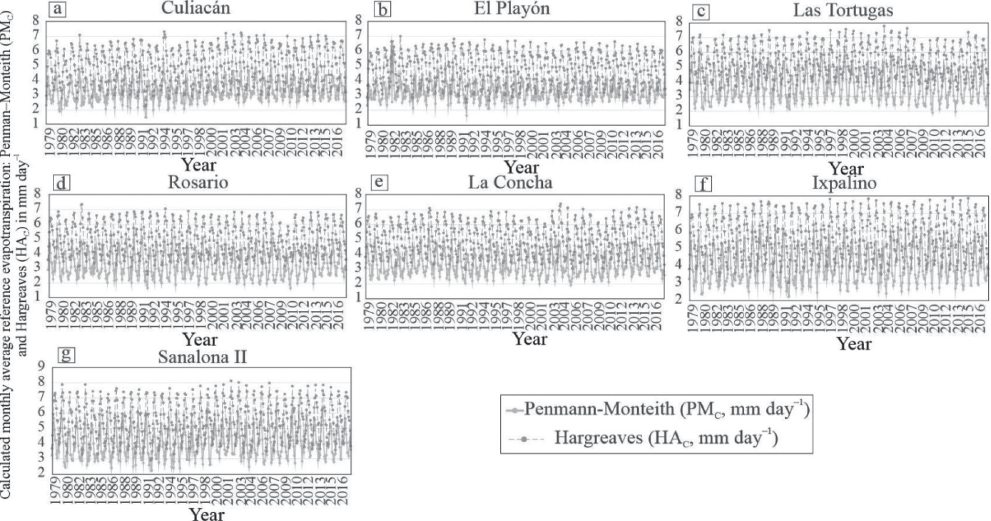
The average ETo ranged from PMC = 1.483 mm day–1 in 1992 (Culiacán–Jan, Fig. 2a)) to PMC = 6.656 mm day–1 in 1982 (El Playón–May, Fig. 2b)); and from HAC = 2.256 mm day–1 in 1991 (Culiacán–Dec, Fig. 2a)) to HAC = 8.133 mm day–1 in 2002 (Sanalona II–May, Fig. 2g)). The results of Fig. 2a) are similar to those reported by [41], who found a range from PMC = 3.0 mm day–1 to PMC = 5.8 mm day–1 for the Culiacán valley in the period 2013–2014. The variation between PMC vs HAC ranged from RMSE = 1.861 mm day–1 (El Playón, Fig. 2b)) to RMSE = 1.972 mm day–1 (Culiacán, Fig. 2a)), that is, ETo presents a tendency towards underestimation of PMC and overestimation of HAC (RMSE > 0.3 mm day–1) [9].
Normality Test for the Calculated Average Reference Evapotranspiration: Penman–Monteith
(PMC) and Hargreaves (HAC) Methods
Monthly (Jan–Dec), Seasonal (Mar–Aug), and Annual (Jan–Dec) Series
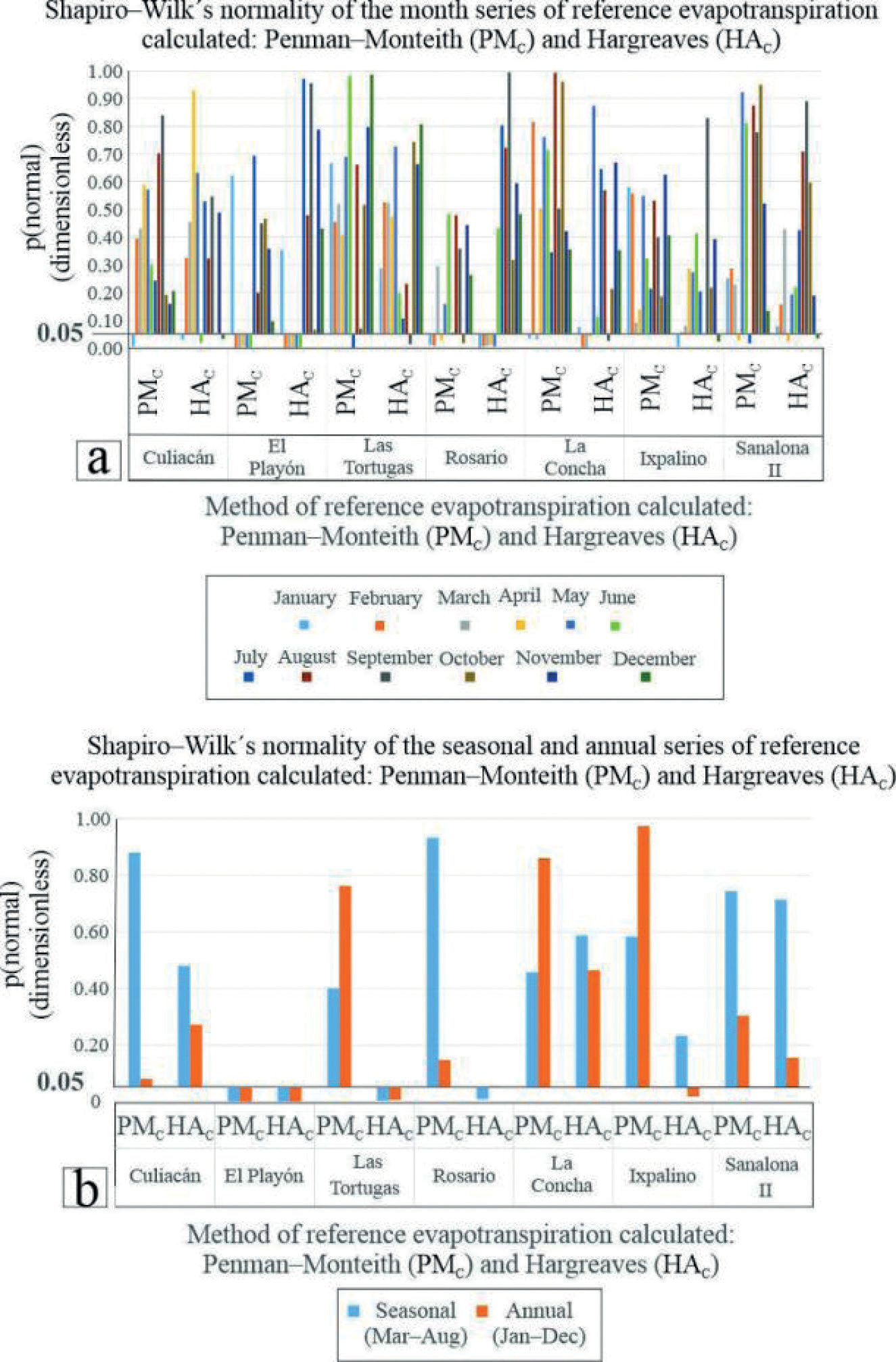
For PMC–Ixpalino in all months (Jan–Dec), p(normal), and W ranged from 0.090 to 0.623 and from 0.951 to 0.978, respectively (Fig. 3a)). In total, 37 monthly series did not present normality; PMC = 15 series and HAC = 22 series (Fig. 3a)). The seasonal series (Mar–Aug) that did not present normality [p(normal) < 0.05] were PMC–El Playón [p(normal) = 7.8×10⁻⁵], HAC–El Playón [p(normal) = 1.7×10⁻⁶], HAC–Las Tortugas [p(normal) = 0.003], and HAC–Rosario [p(normal) = 0.008, Fig. 3b)]. The annual series (Jan–Dec) without normality were PMC–El Playón [p(normal) = 2.3×10⁻⁴], HAC–El Playón [p(normal) = 9.4×10⁻⁷], HAC–Las Tortugas [p(normal) = 0.006] and HAC–Ixpalino [p(normal) = 0.018, Fig. 3b)]. According to [42], the results of the PMC–Ixpalino series (Fig. 3a)) present normality. According to [43], in the results of Fig. 3b), the seasonal series (Mar–Aug) that did not present normality were: PMC–El Playón, HAC– El Playón, HAC–Las Tortugas, and HAC–Rosario, because they did not present the condition of p(normal) > 0.05. According to [43, 44], the annual series (Jan–Dec) that did not present normality were PMC–El Playón, HAC–El Playón, HAC–Las Tortugas, and HAC–Ixpalino, this is due to p(normal) < 0.05.
Pearson (rP) and Spearman (rS) Correlations of Calculated Average Reference Evapotranspiration: Penman–Monteith (PMC) and Hargreaves (HAC) Methods
Monthly Correlations (Jan–Dec)
As shown in Table 2, the correlations ranged from rP = 0.443 (El Playón–Jul) to rP = 0.929 (Las Tortugas– Jan). All rP and rS were significantly different from zero (rP > rcP = |0.316| and rS > rcS = |0.318|). According to [31, 40], the results of Table 2 establish the significant monthly relationship (Jan–Dec) of PMC vs HAC, so monthly modeling of PMR is appropriate (Equations 12–14), applying SLR and SNR, as recommended by [19, 22] and applied by [27, 45].
Seasonal (Mar–Aug) and Annual (Jan–Dec) Correlations
As shown in Table 3, all seasonal (Mar–Aug) and annual (Jan–Dec) rP and rS were significantly different from zero (rP > rcP = 0.316 and rS > rcS = 0.318). Seasonal correlations (Mar–Aug) ranged from rP = 0.693 (Sanalona II) to rP = 0.907 (La Concha). The annual correlations (Jan–Dec) ranged from rS = 0.831 (El Playón) to rP = 0.921 (La Concha). Because all the correlations in Table 3 were significant [31, 40], SLR and SNR can be applied to estimate PMR with a seasonal (Mar–Aug) and annual (Jan– Dec) scale, with HAC as the independent variable [27–45].
Table 2.
Pearson (rP) and Spearman (rS) correlations of the calculated monthly average reference evapotranspiration (Jan–Dec): Penman– Monteith (PMC) and Hargreaves (HAC) methods (dimensionless).
Table 3.
Pearson (rP) and Spearman (rS) correlations of calculated seasonal (Mar–Aug) and annual (Jan–Dec) average reference evapotranspiration: Penman–Monteith (PMC) and Hargreaves (HAC) methods (dimensionless).
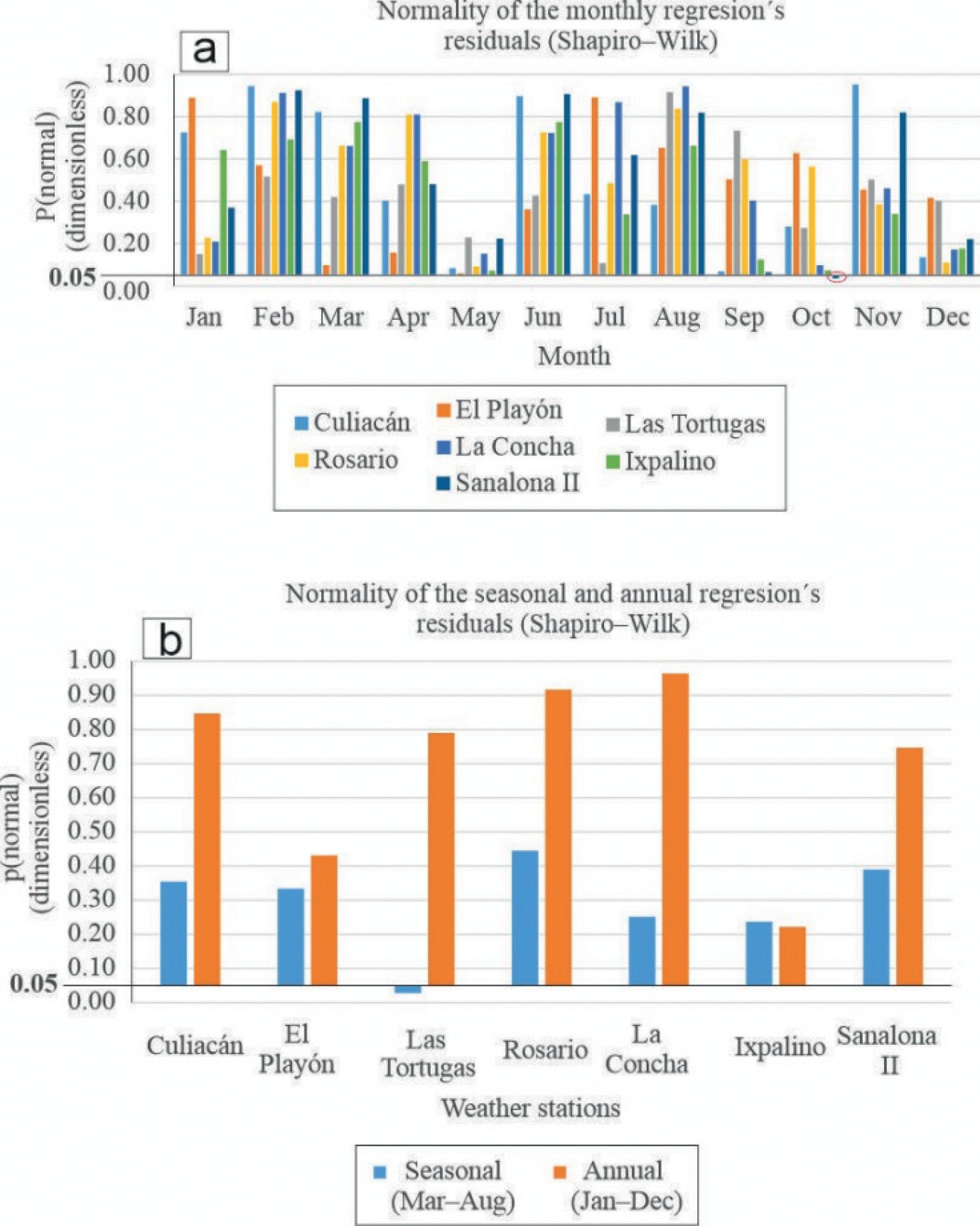
Linear (SLR) and Simple Nonlinear Regressions (SNR) of Calculated Average Reference Evapotranspiration: Penman–Monteith (PMR, dependent Variable) and Hargreaves (HAC, Independent Variable) Methods
Normality Test of Monthly (Jan–Dec), Seasonal (Mar–Aug), and Annual (Jan–Dec) Residuals
The only series of monthly residuals (Jan–Dec) that did not present normality was Sanalona II–Oct [p(normal) = 0.046 and W = 0.942, Fig. 4a)]. In the normal monthly series, the p(normal) values ranged from 0.059 (El Playón–May) to 0.951 (Culiacán–Nov, Fig. 4a)). As seen in Fig. 4b), Las Tortugas for the seasonal period (Mar–Aug) [p(normal) = 0.028 and W = 0.936] was the only series that did not register normality. In the normal seasonal series, the p(normal) values ranged from 0.237 (Ixpalino) to 0.445 (Rosario). In the normal annual series, the p(normal) values ranged from 0.221 (Ixpalino) to 0.964 (La Concha). According to [43] in the results of Fig. 4b), and for the seasonal period (Mar–Aug), the only series that did not present normality was Las Tortugas, because p < 0.05. All series that did present the condition of p > 0.05 were considered normal series [42].
Monthly Coefficients and Goodness of Fit (Jan–Dec)
The fit ranged from R2 = 0.196 (rP = 0.443, El Playón–Jul) with RMSE = 0.274 mm day–1 to R2 = 0.863 (rP = 0.929, Las Tortugas–Jan) with RMSE = 0.218 mm day–1 (Table 4). For the SNR–exponential function (Sanalona II–Oct, Table= 4), R2 = 0.706 (rS = 0.840 > rcS = |0.318|). All RLS (Table 4) exceeded rcP = |0.316| [31, 40] (significant correlation) and did not register a trend towards underestimation or overestimation (RMSE < 0.300 mm day–1) [9]. In Table 4 and for Sanalona II–Oct (SNR–exponential function), the results were rS = 0.840 > rcS = |0.318| [31, 40] (significant correlation) [31, 40]. The methodology of Table 4 was applied to obtain more accurate estimates [19, 22] and was previously applied by [26, 27].
Table 4.
Monthly regression coefficients to estimate calculated reference evapotranspiration: Penman–Monteith (PMR, dependent variable) and Hargreaves (HAC, independent variable) (dimensionless).
Coefficients and Seasonal (Mar–Aug) and Annual (Jan–Dec) Goodness of Fit
Seasonal fit (Mar–Aug, Table 5) ranged from R2 = 0.480 (rP = 0.693, Sanalona II) with RMSE = 0.156 mm day–1 to R2 = 0.823 (rP = 0.907, La Concha) with RMSE = 0.117 mm day–1. Annual fit (Jan– Dec) ranged from R2 = 0.719 (rP = 0.848, Sanalona II) with RMSE = 0.112 mm day–1 to R2 = 0.848 (rP = 0.921, La Concha) with RMSE = 0.082 mm day–1. For the SNR– potential function (Las Tortugas–seasonal, Table 5), the fit was R2 = 0.699 (rS = 0.836 > rcS = |0.318|). All SLR (seasonal and annual, Table 5) exceeded rcP = |0.316| [31, 40] (significant correlation) and showed no trend towards underestimation or overestimation (RMSE < 0.300 mm day–1) [9]. These results are in agreement with [19, 22], who state that PMR models are more accurate than when only Equations 1–10 (PMC) are used. [46] also state that HAC estimation is the most recommended method when data is not available to estimate PMC.
Table 5.
Seasonal and annual regression coefficients, to estimate calculated reference evapotranspiration: Penman–Monteith (PMR, dependent variable) and Hargreaves (HAC, independent variable) (dimensionless).
Validation
Simple Linear Regressions (SLR) between Calculated and Observed Values from: 1) Incident Radiation (SR vs SRg), 2) Penman–Monteith Reference
Evapotranspiration, Calculated with Equations (PMC vs PMO), and 3) Calculated with Regressions (PMR vs PMO)
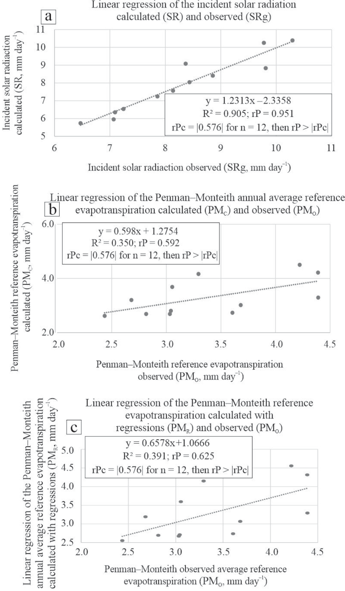
All the monthly average SLR (Fig. 5a)–5c)) recorded rP significantly different from zero (rP > rcP = |0.576|, for n = 12). Specifically for SR vs SRg, the measures of fit were: R2 = 0.905, rP = 0.951, and RMSE = 0.684 mm day–1 (Fig. 5a)). In PMC vs PMO, the measures of fit were R2 = 0.350, rP = 0.592, and RMSE = 0.590 mm day–1 (Fig. 5b)). For PMR vs PMO, the measures of fit were R2 = 0.391, rP = 0.625, and RMSE = 0.578 mm day–1 (Fig. 5c)). The residuals of the three SLR presented normality: p(normal) = 0.193 and W = 0.907 (Fig. 5a)), p(normal) = 0.344 and W = 0.927 (Fig. 5b)), and p(normal) = 0.464 and W = 0.937 (Fig. 5c)). In validation, the three SLRs (Fig. 5a)–5c)) performed well (RMSE < 1.0 mm día–1) [47]. In this study, SR was highly influential (approximately 90.5%) for estimating PMC, which agrees with [8], who points out that SRg in Sinaloa is decisive for the estimation of PMC. According to the results of PMC vs PMO (Fig. 5b)), Equations 1–10 were reliable and sensitive for estimating PMC, even when the series presented missing data [9, 48, 49]. The results of Fig. 5c) and, according to [19, 22, 26, 27], the models of this study are also reliable and sensitive for predicting PMR. Finally, because the residuals of the three SLRs (Fig. 5a)–5c)) presented normality, the SLR is an appropriate statistical tool to use for comparison of calculated and observed data [7].
Conclusions
Due to the lack of data variables from weather stations in Sinaloa, PMC, and HAC were estimated with the use of equations. PMC presented trends toward underestimation, and HAC presented trends toward overestimation. For the first time in Sinaloa, monthly (Jan–Dec), seasonal (Mar–Aug), and annual (Jan–Dec) SLR and SNR were generated to estimate PMR (dependent variable) using HAC (independent variable). Although the equations are a good tool to estimate PMC, the use of PMR estimation models is more precise (without trends of underestimation or overestimation). To try to improve the fit of PMR vs PMO, in future studies, it is recommended to estimate PMR using any other alternative method for ETo, for example, Thornwaite, Priestley–Taylor, Valiantzas, Makkink, Schendel, Jensen, or Turc, among other methods. Knowledge of PMR in Sinaloa can contribute to facilitating the calculation of crop evapotranspiration, which can enable the design of intelligent irrigation plans that are efficient, sustainable, and affordable. The PMR models of this study are also a valuable tool when complete climate series are lacking, which are necessary for the calculation of PMO, since in this study to obtain PMR only latitude– temperature is required. These predictive models can also help ensure, in the near future, the feeding of the population of “the breadbasket of Mexico,” specifically through the relationship between less irrigation water/greater sustainability of food production.