

Introduction
China’s vast rural area is an important spatial carrier of ecology, production, and life. However, in recent years, the extensive development mode has caused great damage to the rural space, causing a series of problems such as the imbalance of rural industrial structure and the deterioration of the ecological environment [1]. China’s extensive rural settlements are distributed in a complex natural environment with undulating terrain, steep slopes, and deep valleys [2, 3]. In recent years, the change in rural landscape patterns has become a hot topic in landscape ecology. With the advancement of new rural construction, the research on landscapes has gradually increased, and many domestic and foreign researchers have made new progress and method innovations in landscape evaluation and protection.
For example, Jin et al. [4] used the Computable General Equilibrium of Land Use Change (CGELUC) and Dynamics of Land System (DLS) models to create a simulation of land use change in Shandong Province in 2025 under three scenarios: baseline, resource consumption, and green development. In the green development scenario, grassland, cultivated land, and unused land are reduced, forest land is basically stable, and water bodies and construction land are increased. There is a downward trend in other scenarios, except for construction land. Land use change is mainly concentrated in the urban periphery, central, and northeast coastal areas, and different scenarios show the overall consistency and local differences.
Teng et al. [5] studied the effects of conservation agriculture and traditional agriculture on soil properties, microbial diversity, and crop yield under 8 years of experimental warming. The results showed that conservation agriculture increased soil organic carbon and microbial biomass carbon under warming conditions, improved soil health by 21%, and increased wheat yield by 9.3%.
Compared to conventional agriculture, conservation agriculture enhances soil resilience to climate change and supports the long-term sustainability of food production. Jing et al. [6] constructed an ecological patch evaluation system for the mainstream basin of the Liao River built on landscape connectivity indicators and morphological spatial pattern analysis and extracted ecological sources. It identified ecological corridors and nodes through the Minimum Cumulative Resistance Model (MCRM) and applied network analysis to comprehensively evaluate the ecological network. This study proposed optimization suggestions and achieved good results. Huang et al. [7] proposed a theoretical framework for transforming Agricultural Landscape Patterns (ALP) in mountainous areas through empirical research in the Caotangxi watershed of the Three Gorges Reservoir area. The ALP of this area was presented in 4 categories: slope farmland orchard conversion, comprehensive conversion, partial and complete abandonment, revealing the various development stages and bidirectional transformation of mountainous agricultural landscapes.
Meanwhile, predicting the changing trends of rural landscapes can help identify areas that may negatively impact the ecological environment and take protective measures in advance. Abbas et al. [8] analyzed the spatiotemporal changes in landscape patterns and structure in the Greater Bay Area. Using fragmentation modeling and structural change analysis, the fragmentation degree of forests, farmland, and grasslands was evaluated, and land use and cover changes were analyzed through the Lorenz curve and Gini index. This method had good landscape pattern prediction performance. Guan et al. [9] constructed an optimization model for the Ecological Security (ES) pattern in the main urban area of Chongqing using the inverse granularity method, MCRM, and spatial network analysis. The optimization results of this study converted non-ecological land into ecological land.
Jahani et al. [10] utilized ANN to model and predict the Aesthetic Quality (AQ) of urban parks and evaluated the esthetic value of 100 urban parks from a user perspective. The study recorded 15 landscape attributes as influencing factors. The maximum coefficient of determination (R²) values on the training, validation, and testing sets were 0.97, 0.88, and 0.90, respectively. The slope of the land and the proportion of flowers, shrubs, buildings, and hard surfaces had the greatest impact on the AQ of the landscape.
Zhang et al. [11] took the Zhaogu mining area as the research object, analyzed the spatiotemporal changes of landscape pattern and ES based on Remote Sensing Image (RSI) classification, and predicted the landscape ES status in 2029. It was found that through the prediction of the Cellular Automata Markov (CA-Markov) model, landscape fragmentation would decrease, connectivity would increase, and the ES situation would continue to improve from 2019 to 2029.
In summary, although there are various methods to simulate and predict landscape patterns, it is difficult for models to fully reflect the complexity of landscape patterns when dealing with large-scale and multidimensional data, especially with nonlinear changes. Many studies have focused on physical changes in landscape structure, ignoring the interaction between ecological functions and socio-economic factors, resulting in limited practical application of optimization proposals. At the same time, the systematic study of landscape patterns in typical karst areas is relatively insufficient, especially since the study of rural landscapes in Guizhou karst areas is rarely reported.
To accurately predict and evaluate the dynamic change of the rural environment in Libo County under the influence of climate change and human activities and put forward the corresponding environmental optimization strategy. Therefore, we use the CA-Markov model to combine the long-term forecasting advantages of the Markov model with the spatial change simulation ability of the CA model to accurately predict the future land use pattern (LUP). However, research on landscape models is still lacking. Therefore, this study innovatively selects Libo County of Guizhou Province as the object and uses CA-Markov to simulate land use change (LUC) in 2030. The evolution trend of regional landscape patterns is analyzed, and the driving factors behind it are revealed, such as population growth and policy change. The study aims to reveal the internal factors of the change of rural landscape patterns in Libo County, provide a reference for ecological landscape planning and beautiful countryside construction, and lay a foundation for further development of rural landscape ecological planning.
Materials and Methods
Overview of the Research Area
Libo County is located in the south of Guizhou Province, under the jurisdiction of the Qiannan Buyi and Miao Autonomous Prefecture, and at the southeast edge of the Yunnan-Guizhou Plateau. The coordinates are between 107°19’ and 107°59’ east-longitude and 25°3’ and 25°45’ north-latitude, with a total area of approximately 2971 km2. The county’s terrain is high in the south and low in the north, mainly characterized by typical karst landforms. The terrain is complex, consisting of intersecting mountains, hills, and river valleys. Libo County has a subtropical monsoon climate, warm and humid, with a mean annual temperature of about 18ºC and an annual precipitation of about 1300 mL. The unique geographical location and climate conditions have created rich biodiversity with high forest coverage. The county has a world natural heritage site - Libo Karst, home to numerous rare animals and plants with extremely high ecological value. The economy is mainly based on agriculture, and in recent years, relying on karst landforms and ethnic minority cultures, the tourism industry here has gradually developed. However, due to the complex terrain, limited land resources, and long-term development, Libo County faces significant ecological pressure. The changes in rural landscape patterns especially pose challenges to ES and sustainable development.
Data Source and Processing
Data sources are as follows. Remote sensing image data were derived from Landsat ETM/OLI images from 1995 and 2020 for land use classification and change detection. The digital elevation model (DEM) is based on the Libo SRTM DEM with a 30 m resolution, using the Gaussian Kruger projection and CGCS2000 coordinate system. The social and economic data came from the Guizhou Provincial Governments’ website, the Guizhou Statistical Yearbook (2000-2020), and the Guizhou Bureau of Statistics. Soil, vegetation, and climate data were collected from relevant literature [12]. It can obtain information about historical changes and folk customs through landscape distribution surveys, resident interviews, and department consultations. The data processing content is as follows: Firstly, the image is preprocessed; that is, radiometric correction, atmospheric correction, and geometric correction are carried out on the remote sensing image to improve the data quality. Second, land use classification. The classification was completed by combining remote sensing images, field investigation, and expert knowledge. Then, the classification results of 1995 and 2020 were compared to analyze the change in land use. After that, attribute data such as area, position, and shape are extracted from the classification results. Finally, the area and distribution characteristics of land use change were analyzed to explore the dynamic evolution of the study area.
Research Method
The land types in the research area are classified. Forest land includes land where trees, shrubs, and bamboo vegetation grow and is used for forestry purposes such as forests and shrubs. Meadow coverage is above 5%, mainly on land where herbaceous plants grow, including pastures, primarily used for grazing and grassland ecological purposes. Construction Land (CL) is used for constructing infrastructure such as urban and rural residential areas, industries, and transportation, including residential and industrial areas in both urban and rural areas. Water encompasses natural water bodies and hydraulic facilities, including lakes, rivers, and reservoirs. Plowland is land used for growing crops, mainly for cultivating crops such as grains and vegetables. Unutilized land refers to undeveloped or difficult-to-utilize land, which may include shrub meadows and sparse forest meadows. As an important component of traditional settlement landscapes, rural residential areas can quantitatively reveal the evolution trends of these features in specific areas through the analysis method of landscape pattern indices. When studying the spatiotemporal changes of rural settlements in ethnic minority areas of Chongqing, key indicators such as the Number of Patches (NP), Class Area (CA), and Patch Density (PD) were selected for analysis [13-15]. These indicators not only reflect changes in settlement size and distribution but also reveal the impact of environmental factors on rural settlement patterns. The single dynamic degree K is utilized to measure the magnitude of change in a specific landscape over a certain period, and its calculation formula is given by Equation (1).
In Equation (1), T is time. Ua is the initial area. Ub is the area at the end. The comprehensive landscape dynamic degree LC is taken to measure the degree of dynamic changes in the landscape during a certain period, as shown in Equation (2) [16, 17].
In Equation (2), Lu is the total area of the landscape within the study area.
In Equation (3), Sij is the transfer area of landscape type from Class i to Class j. n is the total number of landscape types. The standard deviation ellipse reveals the research object’s overall contour and dominant distribution direction [19]. The long and short axes are the distribution direction and range. The greater the difference between the long and short axes, the stronger the directionality. The shorter the half-axis, the higher the data concentration. The long and short axes are used to quantitatively describe spatial distribution characteristics [20, 21]. Landscape index is an intuitive method for quantifying landscape patterns. The hierarchical division of the landscape pattern index is as follows: patch level, type level, and landscape level, covering areas, edges, isolation, aggregation, and other aspects [22]. Table 1 shows the names and indicators of specific landscape pattern types.
NP refers to NP = n, and a larger NP means a higher fragmentation degree. The average CA represents the average area size of each plaque within the study area, and its calculation process is Equation (4) [23].
In Equation (4), A and N are the total area and total number of all plaques within the study area. The calculation of PD is Equation (5) [24].
The expression of the maximum plaque index is Equation (6).
In Equation (6), amax is the area of the largest plaque. The perimeter area fractal index indicates that the patch shape is less irregular or complex, while the opposite indicates that the shape is closer to a simple geometric shape, as shown in Equation (7) [25].
In Equation (7), ln pij and ln aij are the circumference and area values of the j-th part of the i-th plaque after natural logarithmic transformation. The calculation of edge density is shown in Equation (8) [26].
In Equation (8), E is the total length of the plaque boundary. The spread index reveals the clustering and spreading characteristics of the landscape by analyzing the relative area of each patch type and their adjacency relationships. Its calculation expression is Equation (9) [27].
In Equation (9), pi is the proportion of the area of type i plaque to the total area. gik is the adjacency frequency between the i-class plaque and the k-class plaque. m is the total NP types in the landscape. The expression of the aggregation index is Equation (10) [28].
The separation index is Equation (11).
The Cohesion Index (CI) is an indicator used to measure the connectivity and aggregation degree of various patch types in a landscape [29]. It reflects the connectivity of the landscape, that is, whether the patches in the landscape tend to connect and form larger and more coherent landscape units, as shown in Equation (12).
Table 1.
Landscape pattern type names and indicators.
The Shannon Diversity Index (SDI) is an indicator utilized to quantify the species diversity in a community, reflecting the species’ overall richness and evenness. The Shannon Uniformity Index (SUI) measures the degree of uniformity of species distribution in a community, specifically measuring the uniformity of species distribution, and is a standardization of the diversity index [30]. The SDI and SUI are calculated using Equation (13).
The Local Indicators of Spatial Association (LISA) graph is a tool used to analyze LISA properties in spatial data. The LISA diagram visualizes the relationship between each Spatial Unit (SU) and its adjacent units, revealing the local clustering and anomalous data patterns in space. The specific expression of LISA is given by Equation (14).
In Equation (14), I is the LISA index, which measures the degree of correlation between the i-th SUs and its neighboring units. xi is the attribute value of the i-th SUs. X is the average value of all SUs. Si2 is the local variance of the i-th SUs, reflecting the degree of dispersion of the attribute values of the i-th unit and its surrounding units. ωi.j is an element in the spatial weight matrix, representing the spatial proximity relationship between the i-th and j-th SUs. xj is the attribute value of the j-th SUs, corresponding to the i-th unit. By extracting the centroid of settlement points and using nearest neighbor analysis to determine their degree of agglomeration, R>1 is discrete, R = 1 is random, and R<1 is agglomeration. The mean nearest neighbor index is Equation (15).
In Equation (15), A denotes the research area’s area. D0 is the average of the actual nearest distances, which is the average distance between all points in the study area and their nearest neighbors. De is the expected nearest neighbor distance under random distribution conditions. di is the distance between the i-th point and its nearest neighbor. The Average Nearest Neighbor (ANN) value can be used to analyze the distribution of settlements, but it is necessary to use a standardized Z-value test to determine whether the distribution status is significant, as shown in Equation (16).
In Equation (16), Z is the standardized Z-value used to test the significance of the difference between the actual observed values and the expected values. SE is the standard error used to measure the degree of standardization of the difference between observed values and expected values. n is the number of points within the research area. Fig. 1 shows the construction steps of the CA-Markov model designed by the research.
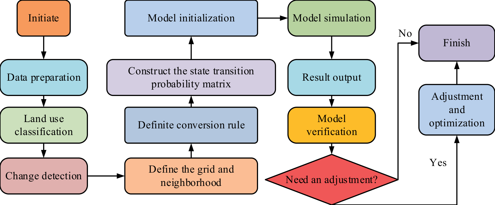
Fig. 1 shows the CA-Markov model construction process. First, Landsat remote sensing images from 1995 and 2020 were collected, and socio-economic data such as population and economic development and natural environment data such as soil, vegetation, and climate were integrated. After radiation, atmospheric, and geometric correction, the images were classified into cultivated land, forest land, construction land, and other types. The characteristics of land use change were analyzed by comparing the classification results of the two periods.
The research area is divided into regular grids, and the local rules are set according to the possibility of land type conversion using the von Neumann or Moore neighborhood. Using the historical data, the transition probability is calculated, the state transition matrix P is constructed, and the initial state is assigned to the grid cells according to the initial data. By combining CA rules and transition matrices, the state changes of grid cells are simulated to generate land use prediction maps and statistical data. Finally, the results are verified by the actual data, and the parameters and rules are adjusted to optimize the model performance. The CA-Markov model combines Markov chains and CA filters to predict LUC and transition probabilities. The function of the Markov model is given by Equation (17).
In Equation (17), Pij is the state transition probability matrix. Cellular automata are composed of regularly arranged grids, with each grid cell referred to as a ‘’cell’’. The expression of the dynamic model is Equation (18).
In Equation (18), N is the neighborhood of the cell. f is the transformation rule for the cellular states in the local space. The Kappa coefficient is a commonly used accuracy evaluation index that can effectively measure the consistency between the predicted results of the model and the actual situation. The Kappa coefficient can be used to detect and evaluate the accuracy of predicting the evolution of regional Land Use Types (LUTs) in Libo County, as shown in Equation (19).
In Equation (19), p0 is the proportion of actual observed values that are completely consistent with predicted values. pc is the expected ratio of observed values to predicted values under completely random conditions. pp is the theoretically perfect consistency ratio, usually 1.
Results and Discussion
Statistical data shows that from 1995 to 2020, the scale of CL in Libo County was relatively stable in the early stage, but due to natural conditions and social development stages, land use expansion was relatively slow. However, in light of the accelerated pace of economic growth and urbanization that characterized the latter period, the scale of CL has undergone a notable transformation. Especially driven by infrastructure construction, industrial layout adjustment, and population growth, the intensity of land development has significantly increased, and the expansion speed of CL has significantly improved. The proportion of CL and forest land in Libo County from 1995 to 2020 is shown in Fig. 2.
In Fig. 2a), the CL area gradually increased from a low level in 1995, especially between 1995 and 2020, with a significant growth rate, rapidly increasing from less than 2 km2 to over 3 km2. Meanwhile, the proportion of CL also increased, indicating that during this period, economic development and urbanization processes accelerated, leading to a significant increase in demand for CL. Fig. 2b) shows the changes in forest land during the same period. Although the total area of forest land remained relatively stable during this period, its proportion fluctuated slightly between 40% and 45% overall. This indicates that despite the expansion of CL, forest land still accounts for a considerable proportion, reflecting the protection and emphasis on the ecological environment during the development process. Fig. 3 shows the changes in the proportion of water and plowland area, as well as the proportion of meadow area in Libo County from 1995 to 2020.
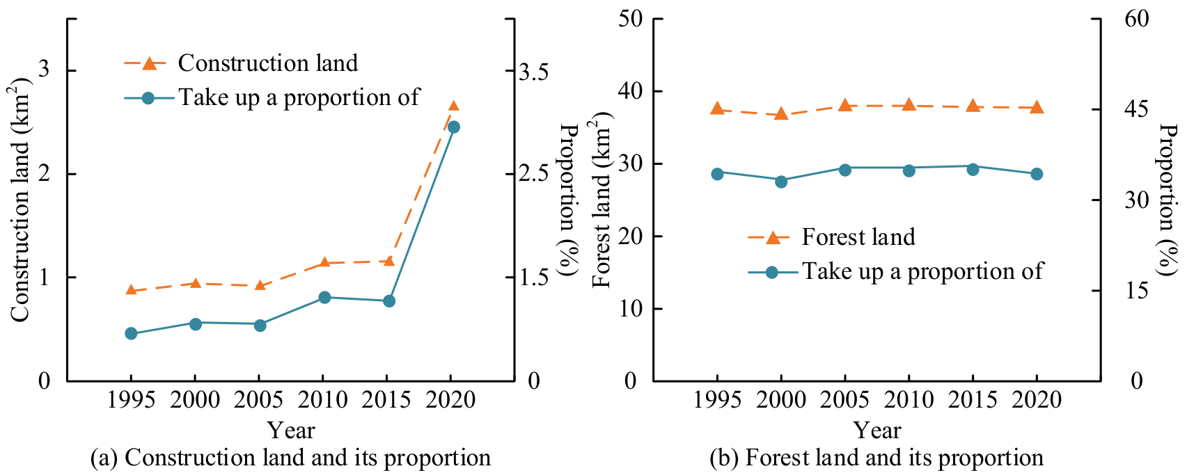
Fig. 3a) shows that from 1995 to 2020, the water area in Libo County remained at around 0.15 square kilometers, accounting for nearly 1%, without significant changes, indicating that water resources are relatively stable. The area of plowland remained around 40 square kilometers throughout the entire period, accounting for 40% to 45% of the total area. Despite slight fluctuations, it remained stable overall, demonstrating the importance of plowland in land use structure. In Fig. 3c), the meadow area was close to 10 km2 in 1995 and 2000, accounting for approximately 10%. However, since 2000, the area of the meadow has significantly decreased, dropping to less than 2 km2 and accounting for less than 2% by 2005. This change may be related to changes in LUPs or increased development activities. From then until 2020, the area and proportion of meadows remained stable at a low level, about 2 km2, accounting for approximately 5%, indicating that meadow resources have not been restored to their previous levels and may be difficult to recover due to long-term impacts. Fig. 4 shows the dynamic degree of single land use in Libo County from 1995 to 2020.
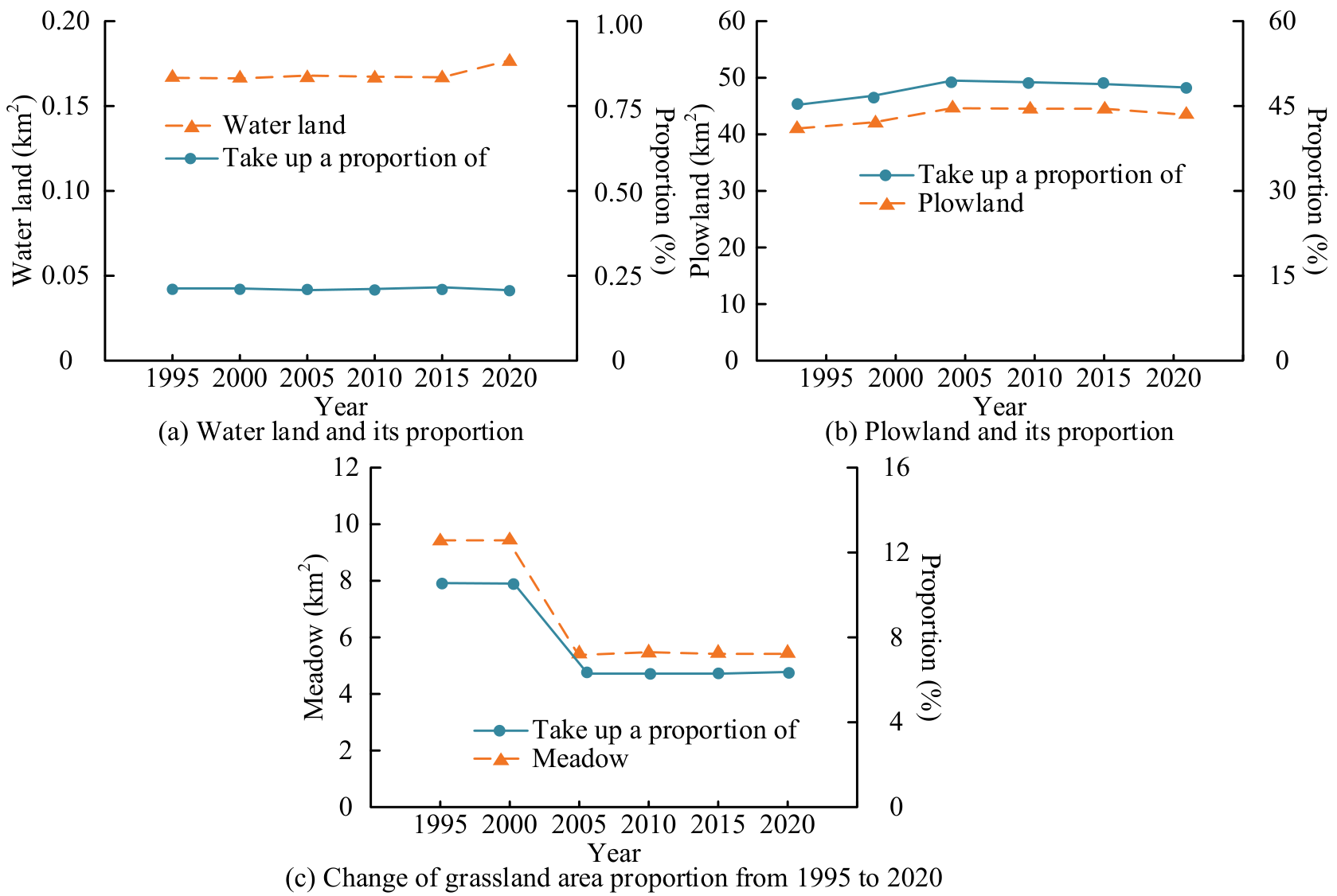
Fig. 4a) shows significant changes in LUTs in Libo County from 1995 to 2020. In Fig. 4b), CL showed significant growth between 1995-2000 and 2005-2010, particularly from 2015-2020, with an increase of 1.50 km2 (30.00%), indicating an accelerating expansion trend. In Fig. 4c), Forest Land experienced a significant decrease of 0.81 km2 (-16.20%) between 1995 and 2000 but recovered to 1.20 km2 (24.00%) between 2000 and 2005, after which it remained relatively stable. In Fig. 4d), the water area remained stable, with only a slight increase of 0.01 km2 (0.20%) between 2015 and 2020. In Fig. 4e), plowland significantly increased by 2.72 km2 (54.40%) from 2000 to 2005 but decreased by 1.21 km2 (-24.20%) from 2015 to 2020, with significant fluctuations. Meadow sharply decreased by 3.92 km2 (-78.40%) from 2000 to 2005 and remained low without significant changes. Fig. 5 is the Comprehensive Land Use Dynamics (CLUD) of Libo County from 1995 to 2020.
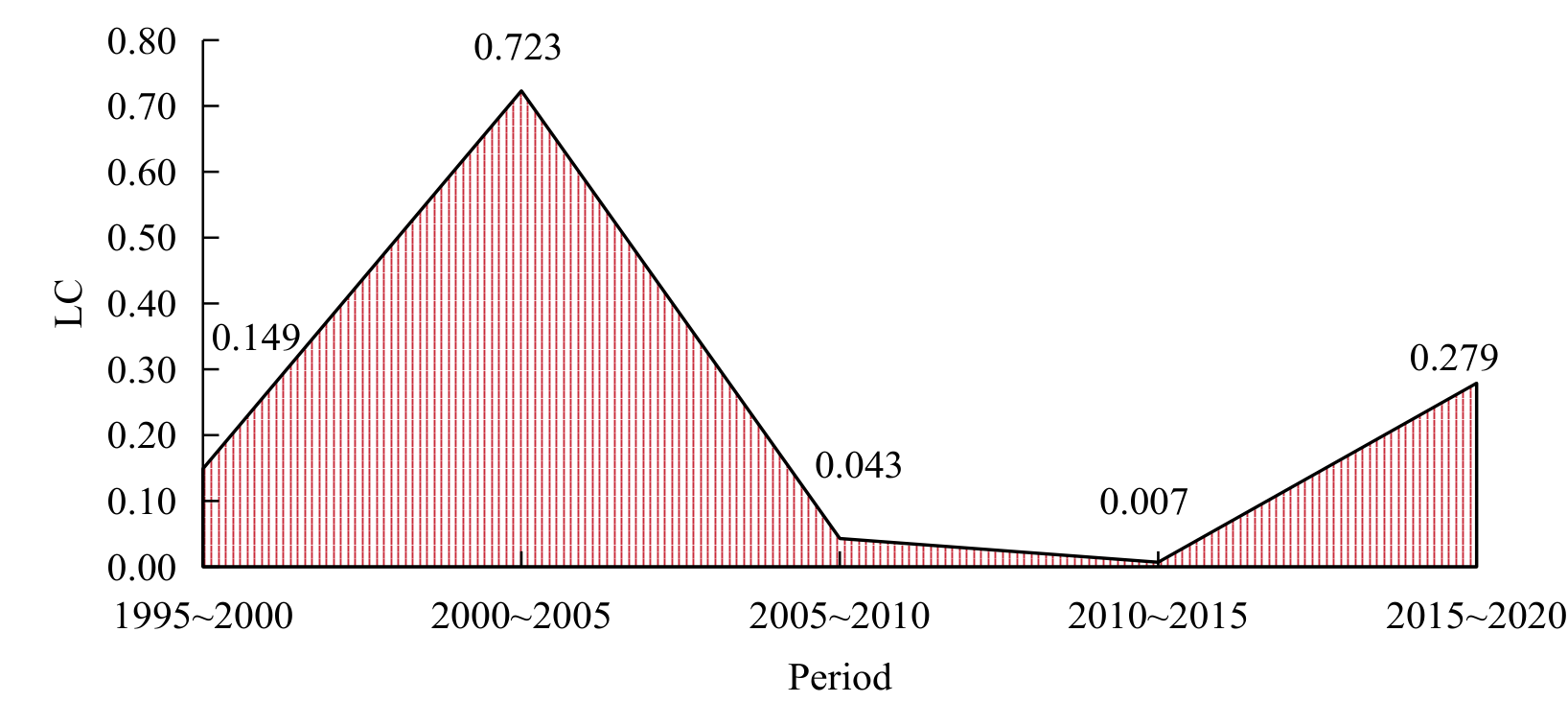
In Fig. 5, the LUC in Libo County from 1995 to 2000 was flat, with a Comprehensive Dynamic Degree (CDD) of 0.149. From 2000 to 2005, the CDD significantly increased to 0.723, indicating that LUC is severe and may be influenced by socio-economic development and policies. From 2005 to 2010 and from 2010 to 2015, the CDD decreased to 0.043 and 0.007, respectively, indicating that the changes tended to stabilize. By 2015- 2020, the CDD had once again risen to 0.279, indicating a certain adjustment in land use. Overall, land utilization presented obvious changes between 2000-2005 and 2015-2020, while other periods remained relatively stable, reflecting the volatility of land use influenced by multiple factors. Fig. 6 shows the dynamic land use transfer matrix of Libo County from 1995 to 2020.
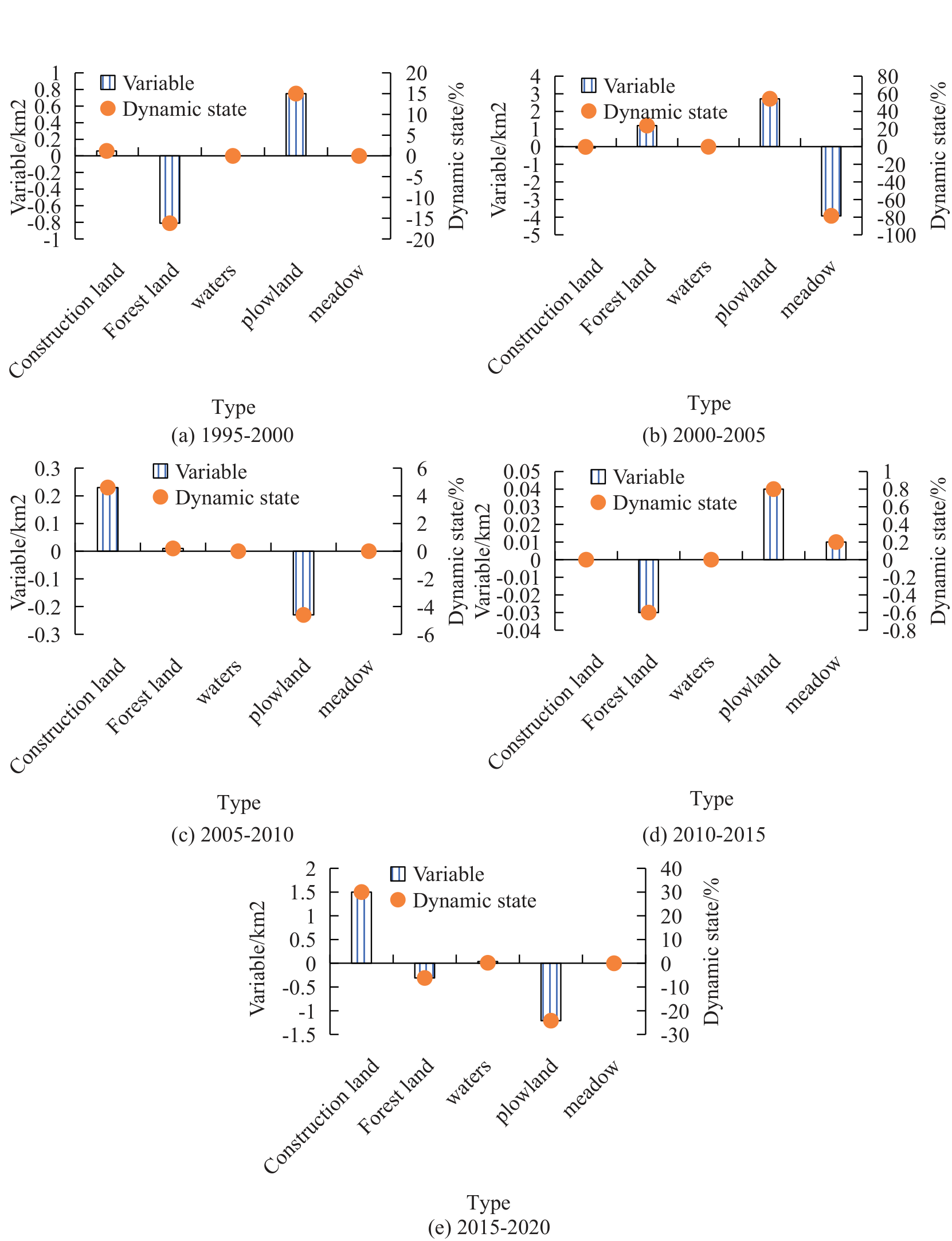
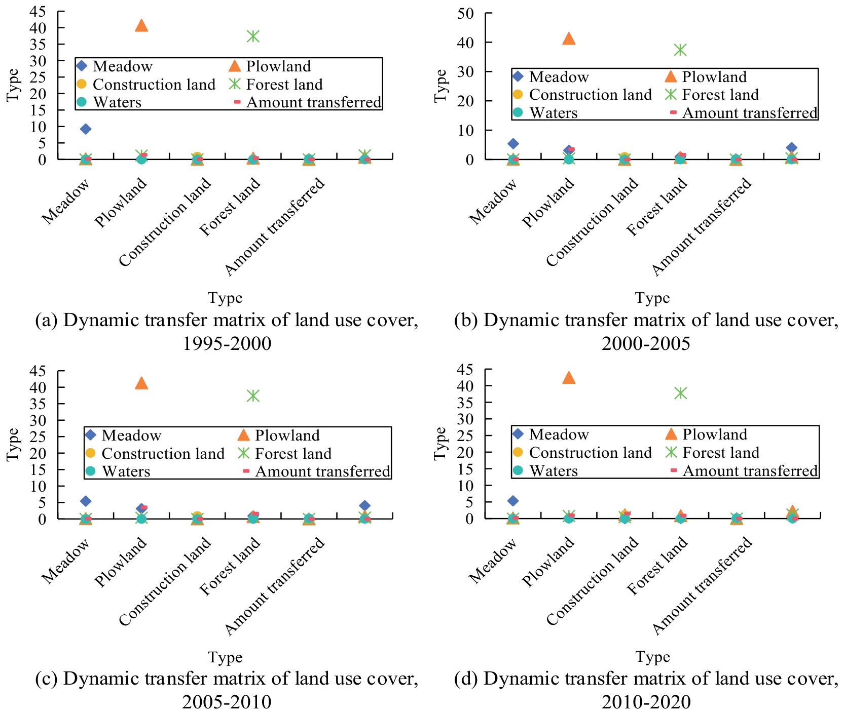
In Fig. 6a), the LUC in Libo County went through several stages from 1995 to 2020. Between 1995 and 2000, LUC was relatively flat, with a CDD of 0.149. In Fig. 6b), from 2000 to 2005, LUC was significant, with a CDD increasing to 0.723 and the mean decreasing by 4.05 km2, mainly shifting to plowland and forest land. Plowland increased by 3.54 km2, forest land increased by 1.62 km2, and CL also saw growth. In Fig. 6c), from 2005 to 2010, LUC tended to stabilize, with a CDD decreasing to 0.043, while the mean and plot remained relatively stable. Meadows decreased by 0.08 km2, while CL and forest land slightly increased. In Fig. 6d), from 2010 to 2015, LUC remained stable with a CDD of 0.007. Meadows decreased by 0.10 km2, plowland slightly decreased, CL increased by 0.03 km2, and forest land increased by 0.383 km2. From 2015 to 2020, LUC intensified again, with the CDD rising to 0.279, indicating that the volatility and adjustment process of land use was influenced by various factors. Overall, LUC was relatively significant between 2000-2005 and 2015-2020, while other periods remained relatively stable. Table 2 shows the standard deviation ellipse of CL in Libo County from 1995 to 2020.
In Table 2, in 1995, the rotation angle of the CL in Libo County was 117.27°, indicating that the spatial distribution direction at that time was consistent with this angle. After 2000, the rotation angle significantly decreased and stabilized at about 28°, indicating a shift in distribution direction. Between 1995 and 2015, the X-axis standard deviation remained relatively stable, but by 2020, it had significantly increased to 3.00 km. The Y-axis standard deviation remained stable after a significant increase in 2000 and increased to 3.91 km in 2020. The CL area rapidly increased from 2.69 km2 in 1995 to 10.12 km2 in 2000, reaching 36.59 km2 in 2020. The circumference also increased from 6.65 km to 21.73 km. This indicates that CL’s expansion speed and scale significantly accelerated between 2000 and 2020, and the spatial distribution underwent significant changes. Table 3 shows the standard deviation ellipse of forest land in Libo County from 1995 to 2020.
In Table 3, the rotation angle of forest land in Libo County remained stable from 36.72° in 1995 to 37.80° in 2020, indicating little change in spatial distribution direction. The X-axis standard deviation fluctuates slightly between 3.42 and 3.57 km, while the Y-axis standard deviation gradually decreases from 5.49 km to 4.87 km, indicating a gradual concentration of forest land distribution. The forest land area decreased from 59.35 km2 in 1995 to 54.38 km2 in 2020, and the circumference decreased from 28.41 km to 26.62 km. This reflects that forest land boundaries have become more regular or their area has decreased. Overall, the spatial distribution of forest land is stable, but the area and scope are gradually shrinking, and the distribution is more concentrated. Table 4 shows the standard deviation ellipse of plowland in Libo County from 1995 to 2020.
Table 2.
CL standard deviation ellipse in Libo County from 1995 to 2020.
Table 3.
Forest land standard deviation ellipse of Libo County from 1995 to 2020.
Table 4.
Plowland standard deviation ellipse of Libo County from 1995 to 2020.
Table 5.
Mean standard deviation ellipse of Libo County from 1995 to 2020.
In Table 4, in 1995, the rotation angle of forest land in Libo County was 46.83°, which increased to 51.32° in 2000 and gradually decreased to 42.23° in 2020, indicating an adjustment in spatial distribution direction. The X-axis standard deviation remained relatively stable from 1995 to 2015, slightly decreasing to 5.01 km in 2020. The Y-axis standard deviation has significantly increased since 2000, reaching 5.87 km by 2020, indicating the expansion of forest land in the Y-axis direction. The forest land area gradually increased from 86.98 km2 in 1995 to 95.43 km2 in 2015 and slightly decreased to 91.97 km2 in 2020, with a corresponding increase in circumference to 34.17 km. Overall, forest land’s spatial distribution, area, and shape have undergone significant changes during this period, particularly in terms of Y-axis direction and area expansion. Table 5 shows the mean standard deviation ellipse of Libo County from 1995 to 2020.
In Table 5, the rotation angle of the meadow in Libo County was 66.17° in 1995, decreased to 64.39° in 2000, reached a peak of 76.98° in 2010, and fell back to 73.18° in 2020, indicating that its spatial distribution direction has undergone fluctuations and adjustments. The X-axis standard deviation remained relatively stable throughout the entire period, slightly increasing from 5.76 km in 1995 to 5.91 km in 2020. The Y-axis standard deviation increased from 3.28 km in 1995 to 3.64 km in 2010 and decreased to 3.37 km in 2020, indicating an expansion of the mean distribution in the Y-axis direction but a slight contraction thereafter. The area of the meadow increased from 59.01 km2 in 1995 to 67.09 km2 in 2010 and slightly decreased to 62.29 km2 in 2020. The circumference also increased accordingly, reflecting the expansion and complexity of the meadow area and boundary shape. Fig. 7 shows the patch situation in Libo County from 1995 to 2020.
In Fig. 7a), the LUP in Libo County has undergone some changes from 1995 to 2020.
The NP of plowland has always been the highest, although slightly reduced; its maximum NP remains at around 40%, indicating the dominant position of plowland in land use. The NP and CI of forest land and meadow in Fig. 7b) were basically stable, with a low maximum NP and little variation. In Fig. 7c), the NP of water was low but fluctuating, with the lowest CI and an increase in 2020. In Fig. 7d), the NP and CI of CL gradually increased, especially significantly in 2020, reflecting the increasing impact of urbanization on land use. The overall CI of various types of land in Libo County remained above 80%, showing high stability, especially the cohesion of plowland and forest land, which was close to 90%, indicating that their spatial structure is relatively stable and there is no obvious trend of dispersion or concentration. Overall, the land use in Libo County exhibited a combination of stability and moderate changes in the process of urbanization. Fig. 8 shows the landscape level landscape pattern index of Libo County from 1995 to 2020.
In Fig. 8a), the maximum NP significantly increased from 1995 to 2005 and then remained relatively stable, indicating the expansion of a dominant land type and occupying a larger area. In Fig. 8b), from 1995 to 2015, the spread index gradually increased, indicating an increase in the expansiveness of land use, but decreased after 2015, which may reflect a trend of land use concentration. In Fig. 8c), the degree of aggregation index significantly increased after 2000, indicating a more concentrated land use, and slightly decreased after 2015, indicating some decentralization of LUPs. In Fig. 8d), the edge density gradually decreases from its high point in 1995, indicating a gradual reduction in the complexity of land use boundaries, possibly due to the concentration of land use. In Fig. 8e), the landscape shape index slightly decreased throughout the entire time period, indicating a trend toward regularizing land use shape. In Fig. 8f) and g), the separation index and SDI have significantly decreased since 2000, indicating a decrease in the diversity and separation of LUTs. In Fig. 8h), SUI significantly decreased after 2000, reflecting an increase in the uneven distribution of LUTs. In Fig. 8i), the fractal index of the perimeter area gradually decreased after 1995, indicating a reduction in the complexity of LUPs. CA-Markov was used to dynamically simulate the land change situation in Libo County in 2030. The land use data from 2000 to 2010 was obtained using Geographic Information System (GIS) software, and its transition matrix was calculated. After obtaining the dynamic transformation of various LUTs over the past decade, the model calculated the distribution probability map of land use. A comparison of the actual results is listed in Table 6.
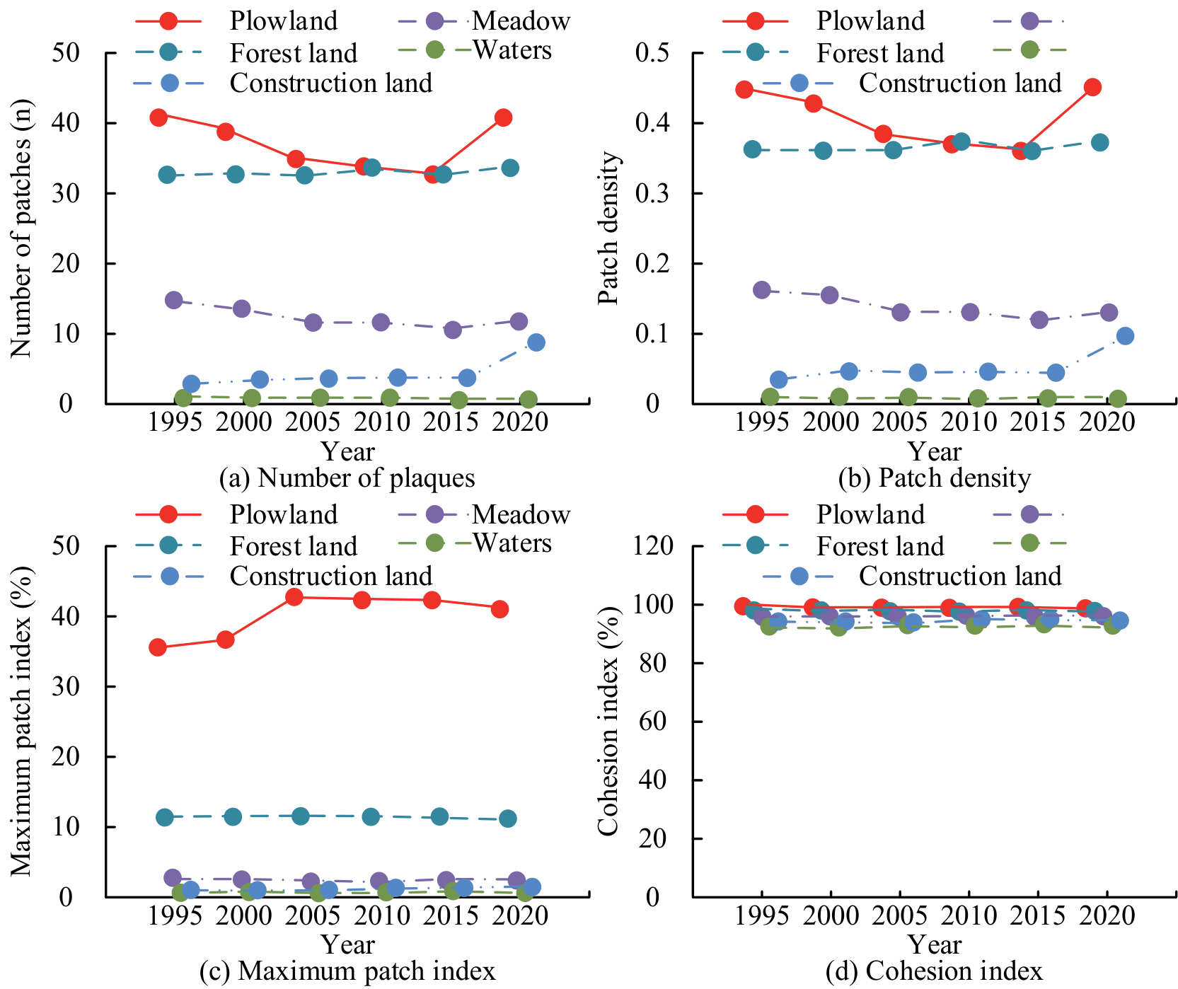
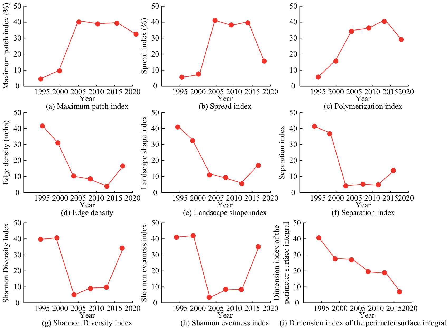
Table 6.
Comparison of land use simulation results in Libo County in 2020.
| Land use type | Simulated area/km | Actual area/ km2 | Relative error/% |
|---|---|---|---|
| CL | 1.90 | 2.67 | 28.19 |
| Forest land | 39.32 | 38.70 | 1.65 |
| Waters | 0.15 | 0.17 | 11.11 |
| Plowland | 45.52 | 43.45 | 4.76 |
| Meadow | 3.55 | 5.53 | 35.74 |
In Table 6, the prediction accuracy of Water and Shadow is relatively high, with errors of 1.65% and 4.76%. The prediction accuracy of plowland is acceptable, with an error of 11.11%. The prediction accuracy for forest land and CL is relatively low, with errors of 28.19% and 35.74%. Overall, the model performs well in predicting water and meadow, but there is room for improvement in predicting forest land and CL. The simulation accuracy of the 2020 LUT map was verified using ArcGIS software. The calculated overall Kappa coefficient was 0.9463. The coefficient is close to 1, indicating that the model has good accuracy and reliability in predicting LUC in 2020. The Conversion of Land Use and its Effects (CLUE) model combines driving factors and policy constraints and uses spatial distribution rules to predict land change. The SLEUTH model, combined with the CA principle, integrated slope, land cover, and other factors to simulate urban expansion. The Future Land Use Simulation (FLUS) model dynamically reflects ecological and socio-economic impacts through cellular automata and multi-objective optimization algorithms. The prediction performance of the research method was compared with that of the CLUE, SLEUTH, and FLUS models, and the results are shown in Table 7.
In Table 7, compared with the CLUE, SLEUTH, and FLUS models, the research model best performs in various indicators. The prediction recall rate (95%), accuracy (92%), F1 score (0.94), and efficiency value (Kappa coefficient 0.95) are all higher than those of other models, and the running time is shorter, and the coverage is wide. Overall, the research model has obvious advantages in accuracy and efficiency. Fig. 9 shows the simulation results of LUTs in Libo County based on the CA-Markov model.
Table 7.
Prediction results of land use change trend and landscape pattern change characteristics of each model.
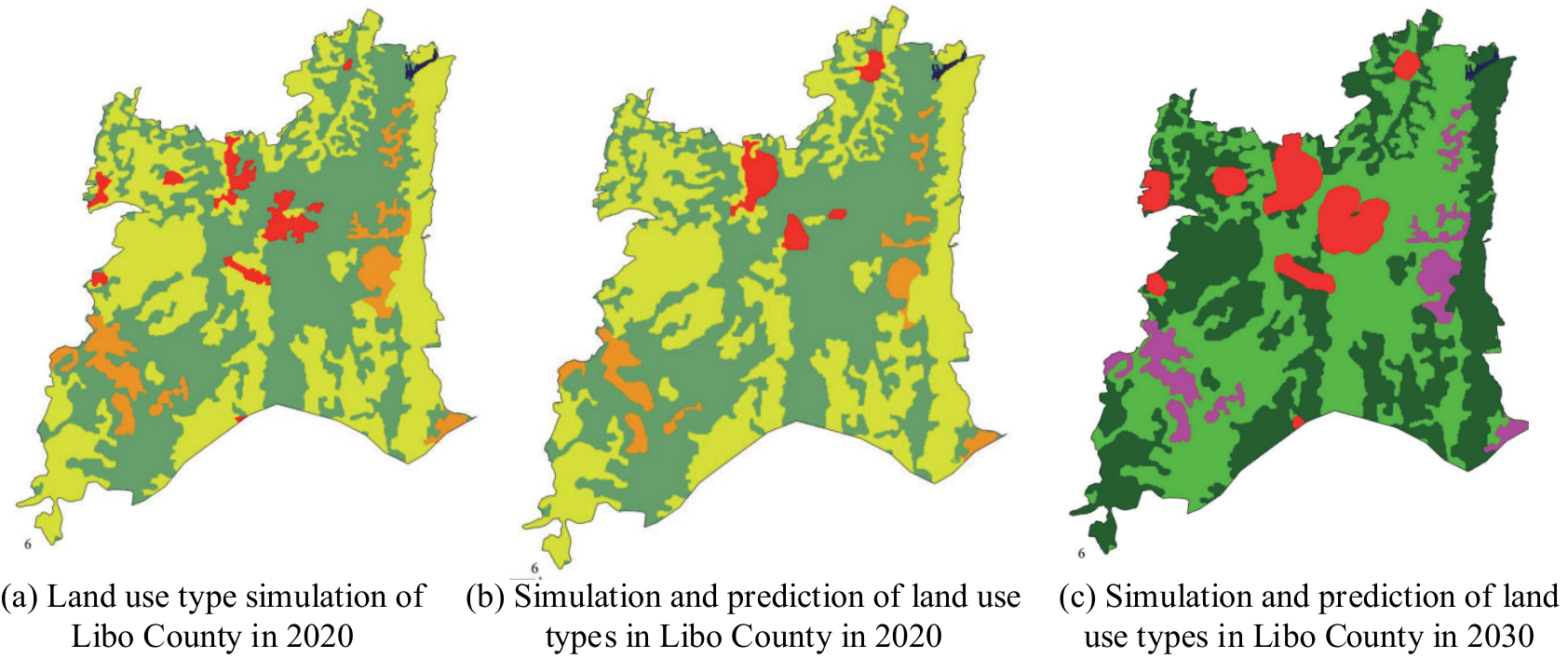
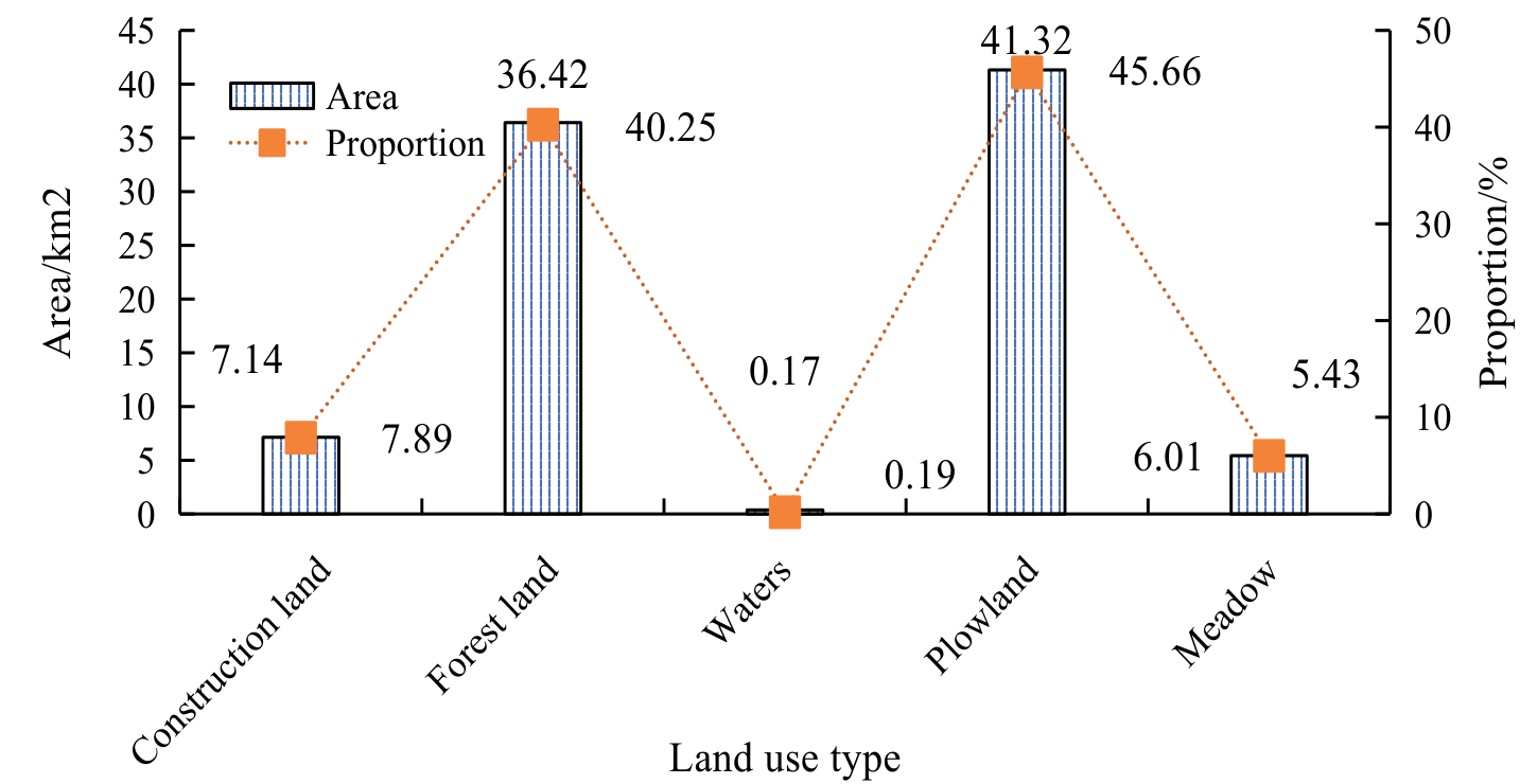
Fig. 9a) shows the simulation results for 2020, Fig. 9b) compares the actual and simulation results for 2020, and Fig. 9c) shows the predicted results for 2030. The analysis shows that the simulation results in 2020 are highly consistent with the actual results, verifying the model’s reliability. Looking ahead to 2030, it is expected that the green area (representing forests or natural vegetation) in Libo County will significantly increase, indicating that there may be increased efforts in ecological protection and vegetation restoration. At the same time, the trend of urban expansion (red areas) has slowed down, which may be related to land use planning policy adjustments. Overall, the LUC trend predicted by the model is in line with the expectations of regional development planning. Fig. 10 shows the simulation and prediction results of land use in Libo County in 2030.
In Fig. 10, the LUTs in Libo County in 2030 are mainly concentrated in plowland and forest land. Plowland covers an area of 41.32 km2, accounting for 45.66% of the total area, and is the main LUT. Next is Forest Land, which covers an area of 36.42 km2, accounting for 40.25% of the total area. The CL covers an area of 7.14 km2, accounting for 7.89%. The meadow covers an area of 5.43 km2, accounting for 6.01%. The water area is the smallest, only 0.17 km2, accounting for only 0.19%. Overall, the land use structure of Libo County in 2030 will continue to be dominated by agricultural land, reflecting the region’s high emphasis on agricultural production and ecological protection in the development process. The land use model based on agriculture indicates that in the future, Libo County will still focus on agriculture and ecological functions, support the goal of regional sustainable development, and maintain the stability and diversity of its ecosystem.
Conclusions
To predict LUC in Libo County, Guizhou, and evaluate its potential impact on the ecological environment, this study combined the CA-Markov model, MCR model, and gravity model. By analyzing Landsat RSIs and DEM data from 1995 to 2020, a land use transfer matrix was constructed to simulate the LUP in 2030. Meanwhile, the impact of landscape changes on ecosystems was evaluated using landscape pattern indices and spatial analysis methods. From 1995 to 2020, the land use change in Libo County is remarkable, especially in construction and cultivated land. Construction land area has nearly tripled, reflecting rapid economic development and urbanization, significantly increasing demand for residential and industrial land.
The overall area of forest land is stable, and the distribution is gradually concentrated, which shows that the ecological protection measures have achieved results. The meadow area has decreased significantly since 2000, revealing the vulnerability of its ecosystem and the impact of land development activities.
The water area remains stable, reflecting the sustainability and effectiveness of water resources management. According to the CA-Markov model, by 2030, the land use of Libo County will still be mainly cultivated land (45.66%) and forest land (40.25%), construction land (7.89%), grassland (6.01%), and water area (0.19%). The continuous expansion of construction land brings economic pressure, and the stability of forest land proves the effective implementation of ecological protection.
The fluctuation of cultivated land area may be related to the change in agricultural policy and market demand, while the decrease in grassland may be caused by the adjustment of development and land use policies. Land-use change poses challenges to ecosystems, biodiversity, and sustainable development while affecting rural economic structures and development patterns.
Based on the research on Libo County, the following suggestions are proposed: Firstly, the ecologically important hilly and mountainous forests should be strictly protected, and land protection should be strengthened. By optimizing the land use structure of townships through rational planning and promoting the redevelopment of existing CL, utilization efficiency can be improved. Urban development should prioritize the protection of ecological diversity, formulate appropriate development intensity strategies, and advocate for low-density and balanced development on site. Meanwhile, it should resolutely implement ecological protection, preserve farmland, and delineate and strictly enforce the red line for protecting basic farmland. It should also strengthen the protection of water resources, delineate red lines for protection in accordance with national regulations, promote the construction of forest and grass vegetation, clarify the scope of protection, and continuously improve the ecological environment.
Land-use change poses challenges to ecosystems, biodiversity, and sustainable development while affecting rural economic structures and development patterns. Remote sensing image data, social and economic data, and natural environment data provide abundant information, but there may be time lags and spatial resolution limitations. The prediction result of the CA-Markov model is highly consistent with reality, which verifies its reliability. The research not only contributes to the academic community but also has important practical significance in the field of practice, especially in formulating and implementing land management and environmental protection policies.