

Introduction
Crop growth is a complex process affected by climate as well as by environmental and field management. The crop model contains many parameters and integrates agricultural science and information technology to simulate the growth process of crops. The crop model has become a crucial resource for conducting research and managing agriculture, ecological, and environmental aspects. Currently, the primary emphasis of its use at a global level has been on the DSSAT model [1-4], the FAO crop model for predicting yield response to water (AquaCrop) model [5-15], the APSIM model [16-18] from Australia, the WOFOST model [19-21], the GECROS model from the Netherlands, and the ORYZA rice model from the Netherland [18, 22]. Crop models play a pivotal role in bolstering agricultural productivity, optimizing resource allocation, and advancing sustainability in agriculture. The significance of these models in contemporary agriculture is progressively highlighted amidst the challenges presented by climate change and the pressing need for resource efficiency [23].
The crop model can support decision-making related to crop field management because it can dynamically simulate and monitor crop growth processes using a series of mathematical formulas [24]. Most researchers appreciate this approach, and the application of it is becoming more extensive. However, the crop model usually needs the input of many parameters, such as climate conditions, plant parameters, field management parameters, soil type, amounts of water and fertilizer, crop varieties, etc. [25]. The crop model also includes many biological and physical processes [26]. Unfortunately, many input parameters have uncertainties, and there are uncertainties in deciding on the model structure, parameter diversification, and identifying the driving factors that cause errors; these issues combined lead to uncertainty in model predictions. It would be highly valuable in crop management to be able to identify how to reduce the uncertainty in the process of crop model prediction and how to reduce the number of input parameters and improve the model prediction accuracy [2, 14]. The calibration of crop model parameters is a crucial step before a crop model is applied to a local area and the process is very complicated [27]. Some crop parameters will change with environmental conditions, local crop varieties, and other factors. Some parameters are responsible for critical processes and the model’s output, and some are insensitive to the output variables of the crop model [28]. Therefore, it is not necessary to calibrate all unknown parameters in the model calibration process, and only a few high-sensitivity parameters need to be calibrated and optimized. Then, the low-sensitivity and zero-sensitivity parameters can be set to fixed values to reduce the difficulty of model calibration [2].
There are two main approaches to consider when conducting sensitivity analysis: local sensitivity analysis (LSA) method and global sensitivity analysis (GSA) method [29]. LSA is most applicable when working with models that are linear or closely resemble linearity, which respond to the relationship between the output variable and input variable, keeping other inputs unchanged [30]. The GSA method is well-suited for complex nonlinear models that involve a large number of input parameters, as it takes into account the impact of multiple changes in parameters and the interdependence between parameters on the output variables of the model [2]. At present, the GSA methods (such as the Morris method) and methods based on variance are widely used. The screening method is suitable for finding a few valid parameters among many parameters because it calculates the average effect on the model simulation results based on changes in a single parameter [31]. Methods based on variance require an extensive model evaluation and are more computationally intensive, and it is possible to calculate both first-order and higher-order sensitivity indices with them [32], such as the Sobol’s method [33], the Fourier amplitude sensitivity test (FAST) method [34], and the extended Fourier amplitude sensitivity test (EFAST) method [35, 36]. The FAST method cannot calculate higher-order exponents. It is possible to gauge the effects of parameter variations on the output of a model using the EFAST method, by utilizing the EFAST method, it is possible to assess the effect of individual parameter variations on the output of a model [14, 26].
To research the uncertainty of parameter sensitivity analysis at the regional scale, a great deal of research has been done in this area by scholars. Li et al. [2] and Ma et al. [37] used the EFAST method to analyze parameter sensitivity in the DSSAT-CERES model, based on their findings, the parameter bounds had little effect on parameter sensitivity. Liu et al. [35] used EFAST to analyze WOFOST parameter sensitivity based on 8 climate conditions, a number of parameters’ sensitivity indexes were observed to be influenced by climate conditions, for example, the parameters SPGF, WGRMX and RGRLMX. Yu et al. [38] conducted an assessment of parameter sensitivity for the ORYZA model within the Yangtze River Basin, and they screened the parameters with a high degree of sensitivity pertaining to paddy rice cultivation. Yang et al. [15] used the Morris and EFAST methods to analyze the global sensitivity of crop (corn, soybean, and winter wheat) yield and transpiration from the AquaCrop model for dry land environments. The study covered three dryland agricultural regions with different climatic conditions. The results showed that parameter sensitivities varied with target model outputs (e.g., yield, transpiration) and humidity conditions. However, most crop model parameter sensitivity analysis studies focus on one or several crops in a particular area. There are few studies on the differences between the sensitivity parameters in different regions or climates. Few studies have analyzed the impact of the environment on the sensitivity differences of crop parameters. To address this gap in the data and in understanding, this study employed the EFAST method to examine how sensitive crop parameters in the AquaCrop model are to biomass and crop canopy coverage (CC), as well as to investigate winter wheat yields under varying climatic conditions. The following main producers of winter wheat in Henan Province, China, were selected for study: Zhengzhou, Anyang, Shangqiu, Luanchuan, Nanyang, Xuchang, Zhumadian, and Xinyang. The study objectives included reducing model input difficulties, exploring crop parameter sensitivity differences under different climate conditions in different regions, and providing technical support for a localized application of the model in Henan Province, China.
Material and Methods
Research Area Overview
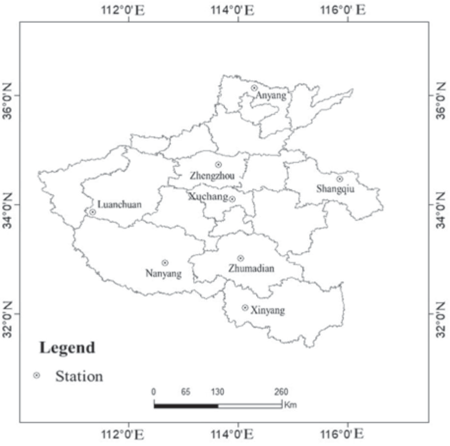
Situated in the central region of China, Henan Province spans a total area of 167000 km2, Located between 31°23’ and 36°22’ north latitude, 110°21’ and 116°39’ east longitude. The majority of the region falls within the warm temperate zone, with the southern portion extending into the subtropical zone, in the northern subtropics and warm temperate zones, a continental monsoon climate dominates. Moreover, there is a climate gradient from low-lying plains to high-elevation hills and mountains, progressing from east to west. The region experiences four distinct seasons, characterized by simultaneous rain and heat, varied and intricate weather patterns, as well as frequent meteorological disasters. The average annual temperature in Henan Province ranges from 10.5ºC to 16.7ºC, while the annual average precipitation spans from 407.7 mm to 1295.8 mm, progressing from south to north. The period from June to August receives the highest amount of rainfall, while the annual average sunshine ranges from 1285.7 to 2292.9 hours, and the frost-free season lasts between 201 to 285 days, providing favorable conditions for cultivating a diverse range of crops. As a crucial grain production hub in China, Henan Province serves as the primary production region for winter wheat. In order to investigate the sensitivity of crop parameters in AquaCrop model under diverse climatic conditions, the study area comprised eight regions, namely Zhengzhou, Anyang, Shangqiu, Luanchuan, Nanyang, Xuchang, Zhumadian, and Xinyang. The research focused on conducting the GSA of the AquaCrop across varying meteorological conditions.
In the transitional zone between the warm temperate and subtropical zones, Henan Province experiences a continental monsoon climate characterized by distinct seasons, simultaneous rain and heat, and a complex, diverse climate. This region is climatically divided into seven zones: northeastern Henan (including Zhengzhou, Xuchang, Shangqiu, Anyang), the western Henan mountainous area (Luanchuan), the Nanyang basin (Nanyang), the southern Huaihe River area (Zhumadian, Xinyang), the northern Huaihe River plain, and central-southern and central-northern Henan. The study focuses on four distinct climatic zones, each exhibiting significant spatial and temporal variations in meteorological factors such as temperature, precipitation, sunshine, and relative humidity. These variations influence the agronomic traits of winter wheat, including growth period, rate, and dry matter accumulation, subsequently affecting the crop’s yield level and stability. Under a continental monsoon humid climate, the northeastern Henan zone has mild weather with distinct seasons and concurrent rain and heat. Winter wheat here has a shorter growth period, faster rate, higher yield, and lower stability and is susceptible to drought, waterlogging, lodging, diseases, and pests. The western Henan mountainous zone, also under a continental monsoon climate, is characterized by cool, rainy weather and ample sunshine, leading to a more extended wheat growth period, a slower rate, and lower yield. With its warm, humid climate and concurrent rain and heat, the Nanyang basin supports a more extended growth period, moderate growth rate, and higher winter wheat yield. Lastly, the southern Huaihe River zone, marked by a warm, dry climate and sufficient sunshine, sees a shorter growth period and faster rate of winter wheat growth but lower yield, with vulnerability to drought, waterlogging, high temperatures, diseases, and pests.
AquaCrop Model
The AquaCrop model, which prioritizes free water productivity, was developed by the FAO in 2009 [6-8]. This model consists of four fundamental components, including meteorological, crop, management, and soil modules, all working together to simulate the influence of water supply on crop yield and biomass. Its significance lies in its ability to facilitate crop production and yield in regions of Africa and Asia where water shortages significantly limit agricultural output. In the AquaCrop model, evapotranspiration is split into two components: crop transpiration (Tr) and soil evaporation (E). The former is inversely proportional to soil vegetation coverage, while the latter is closely related to crop canopy coverage (CC).
Crop transpiration:
where Ks is the soil moisture correction coefficient; Kcbx is the scaling factor of the crop transpiration coefficient; CC* is the adjusted crop canopy coverage; and ET0 is the potential crop transpiration.
Biomass:
Where B is biomass; Ksb is the temperature stress coefficient;Tri is crop evapotranspiration on the day I; and ET0i is the reference evapotranspiration on day i.
Yield (Y):
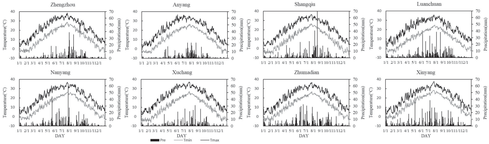
where HI0 is reference Harvest Index;and fHI is the coefficient of adjustment reflects the effects of water stress and temperature stress on crop yields. The data used in the AquaCrop model simulation process was downloaded (http://data.cma.cn/), included the maximum and minimum temperatures, the rainfall, the humidity, the sunshine hours, the atmospheric pressure and the wind speed each day (Meteorological data are shown in Fig. 2). The crop parameters are shown in Table 1.
The EFAST Method
EFAST is a GSA technique developed by Saltelli et al. [39, 40] that combines the advantages of the FAST [41] and Sobol’s methods [42]. This method can analyze the global sensitivity index of input parameters with respect to the output variable variances; the higher the sensitivity index value, the stronger the parameters’ sensitivity. The main formula is described below.
Suppose the y = f (x1, x2, …, xm), and Fourier transform is performed on it. Then, the conversion function is:
where Ai and Bi are the Fourier amplitude, i is the Fourier transform parameter.
where Ns is sample size,
The output variance Vi can be calculated from ωi:
Variance V(Y) can be decomposed as follows:
where Vij-V12…m is the variance of parameter interaction.
Si is the first-order sensitivity index:
STi is the total-order sensitivity index:
Table 1.
Upper and lower values of crop parameters in AquaCrop model.
Parameter Selection and Simulation Methods
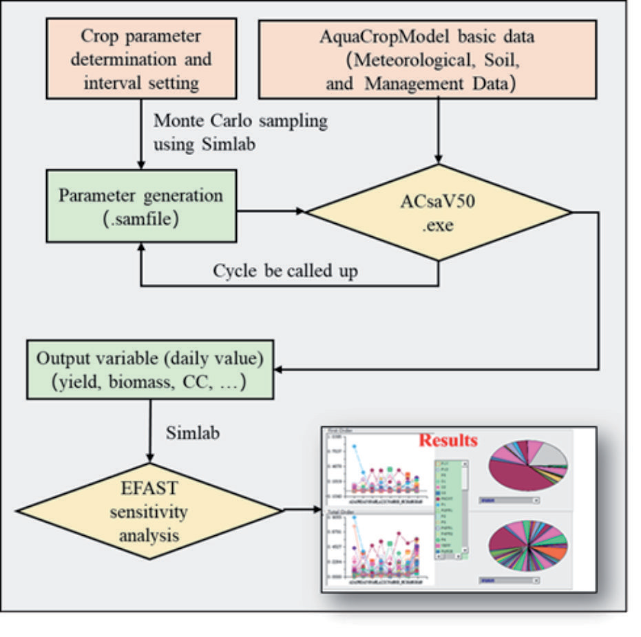
Using the eight regions, namely Zhengzhou and Shangqiu, as the focal areas of investigation, we conducted an analysis utilizing the AquaCrop model to assess the biomass, crop coefficient (CC), and yield of winter wheat based on meteorological data averages spanning the years 2017 to 2020. The EFAST method was employed to scrutinize the sensitivity index and various crop parameters. A comprehensive set of 42 crop parameters was designated as the input parameters file, as presented in Table 1. The software Simlab (Version 2.2.1) was used to perform the global sensitivity analysis. The steps were as follows:
(1) Used Simlab software to generate crop parameters based on the ranges given in Table 1, and assumed that the parameters were uniformly distributed and independent of each other;
(2) Applied the Monte Carlo method to randomly sample 4850 data sets from the parameter ranges;
(3) Wrote the sampled parameters into the AquaCrop model file and used the plug-in ACsaV50 to run the model in batch mode, then organized and summarized the simulation results to obtain the output variables of interest, such as biomass, CC and yield;
(4) Performed sensitivity analysis using the Simlab software to evaluate how the output variables responded to the changes in the input parameters.
AquaCrop’s parameter sensitivity analysis flow chart is shown in Fig. 3.
Results and Analysis
Fig. 4-15 show the sensitivity analysis results for biomass, CC, and yield for winter wheat. The selection of the final SI is based on the first-order sensitivity index (FOSI) FOSI>0.05, and the total-order sensitivity index (TOSI) TOSI>0.1. We selected the SI parameter that meets the above criteria as the final sensitivity parameter. The SI based on the time series (days after planting (DAP)) was the SI value of the first day, and the biomass and CC were selected from winter wheat’s growth period. The yield production was mainly in the late grain-filling period, so the yield SI was set to be 50 days before the winter wheat harvest. The sum of the SI is the sum of the daily SI during the period of winter wheat’s growth. From this work, we selected the SI and the highest six parameters that would best allow us to study the overall performance of crop parameters in the winter wheat growth process. The results are shown in Fig. 7, 11 and 15.
Sensitivity Analysis of Crop Parameters for Winter Biomass
The Final Sensitivity Index
The parameter sensitive to biomass is shown in Fig. 4. Considering the differences of sensitivity parameters in different regions, six parameters were selected, including wp, stbio, kcb, mcc, rtx, and psen. Overall, the sensitivity parameters selected according to FOSI and TOSI were consistent, and the two most sensitive parameters were wp and stbio. The SI of the other four parameters was inconsistent in different regions. The sensitivity parameters were kcb and mcc in Shangqiu, Luanchuan, Nanyang, Zhumadian, and Xinyang; rtx and mcc in Zhengzhou and Xuchang; and rtx, psen, and kcb in Anyang. The parameter rtx was greatly affected by climatic conditions.
The Temporal Dynamics of FOSI Throughout the Growing Season
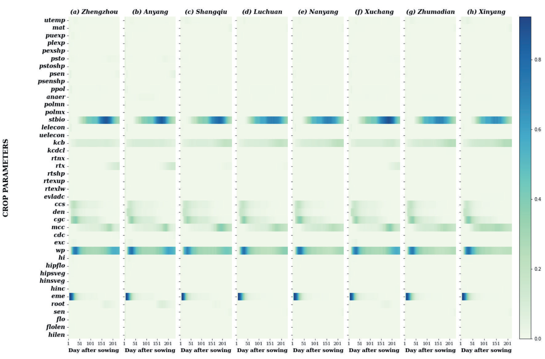
The temporal dynamics of FOSI on winter wheat biomass throughout the growing season are shown in Fig. 5. From the results, the distribution consistency of the SI values was high. The three most sensitive parameters were stbio, wp, and kcb; in addition, the parameters mcc, eme, cgc, ccs, and den also significantly influenced the biomass of winter wheat. The parameter stbio was more significant than 0.1 from about 50 days after planting (DAP) to the harvest; the SI was at its maximum value at about DAP 180, and the maximum SI value was 0.9, which indicated that the parameter had a significant effect on biomass during this period. However, the SI value of parameter stbio differs in different regions. The SI parameters, wp and kcb, were higher in the growing season. The SI value of parameter mcc was higher during DAP 170 and 210, eme was higher during DAP 0 and 30, and cgc was higher during DAP 20 and 50. The SI values of other parameters (such as ccs and den) were higher only in a particular growth stage.
The Temporal Dynamics of TOSI Throughout the Growing Season
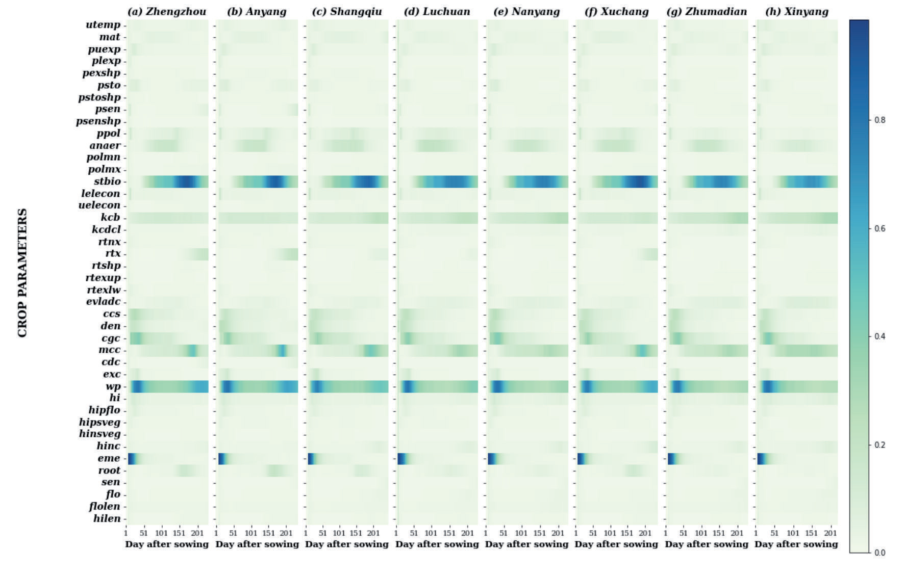
The temporal dynamics of FOSI is shown in Fig. 6. Compared to Fig. 5, the influence of parameter interactions is considered during the GSA, and there are more sensitivity parameters. The three most sensitive parameters were stbio, wp, and kcb. Parameter stbio was more highly sensitive from DAP 50 to the end of the growth period. The sensitivity of parameters, wp and kcb, was high throughout the growing season. Especially for parameter wp, whose SI value was between 0.2 and 0.6, there were some differences between regions. The SI value of parameter mcc was high in late winter wheat growth, and eme was high in early winter wheat from emergence to DAP 50, and other parameters (such as cgc, den, ccs, anaer, ppol, root, and mat) were higher during the winter wheat reproductive periods.
Sum of Sensitivity Index
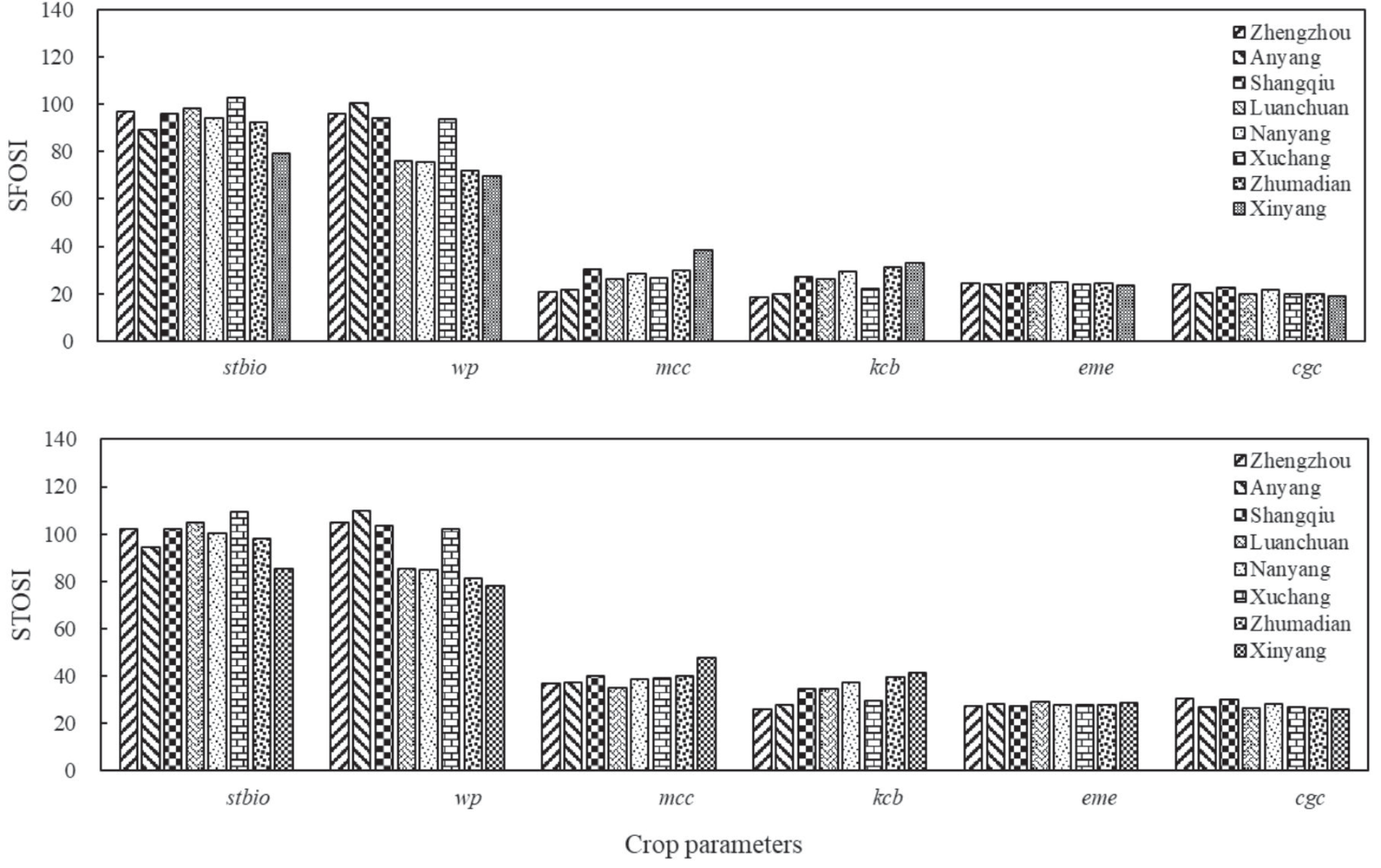
The sum of the first-order sensitivity index (SFOSI) and the sum of the total-order sensitivity index (STOSI) for biomass are shown in Fig. 7. Regarding sensitivity index selection, the highest six parameters of SFOSI and STOSI were stbio, wp, mcc, kcb, eme, and cgc. Parameters stbio and wp were the most sensitive, and the SI sum values were much higher than other parameters. The SI sum values of other parameters (such as mcc, kcb, eme, and cgc) were high, and there were some differences in different regions as well as differences in the sorting of SFOSI and STOSI in the same area.
Fig. 4.
Sensitivity analysis results of crop parameters for winter wheat biomass. FOSI – first order sensitivity indices, TOSI – total order sensitivity indices, Guide was 0.1 reference line.
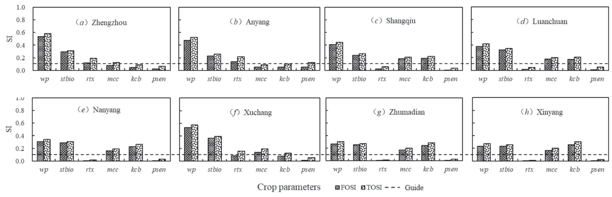
Fig. 5.
First-order sensitivity indices for a time series on winter wheat biomass throughout the growing season.
Sensitivity Analysis of Crop Parameters on CC
The Final Sensitivity Index
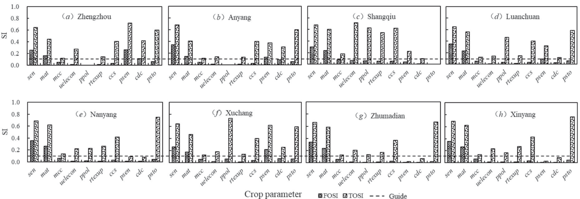
The parameter that was sensitive to biomass is shown in Fig. 8. Overall, the results of FOSI and TOSI were quite different. There were 3-5 parameters with FOSI>0.05: sen, mat, mcc, psen, and cdc, respectively. There were many parameters with TOSI>0.1 [43]: sen, mat, psto, uelecon, ppol, ccs, rtexup, psen, mcc, and cdc, respectively. Parameters sen and mat were the most sensitive in common, but the order of other parameters is irregular
The Temporal Dynamics of FOSI Throughout the Growing Season
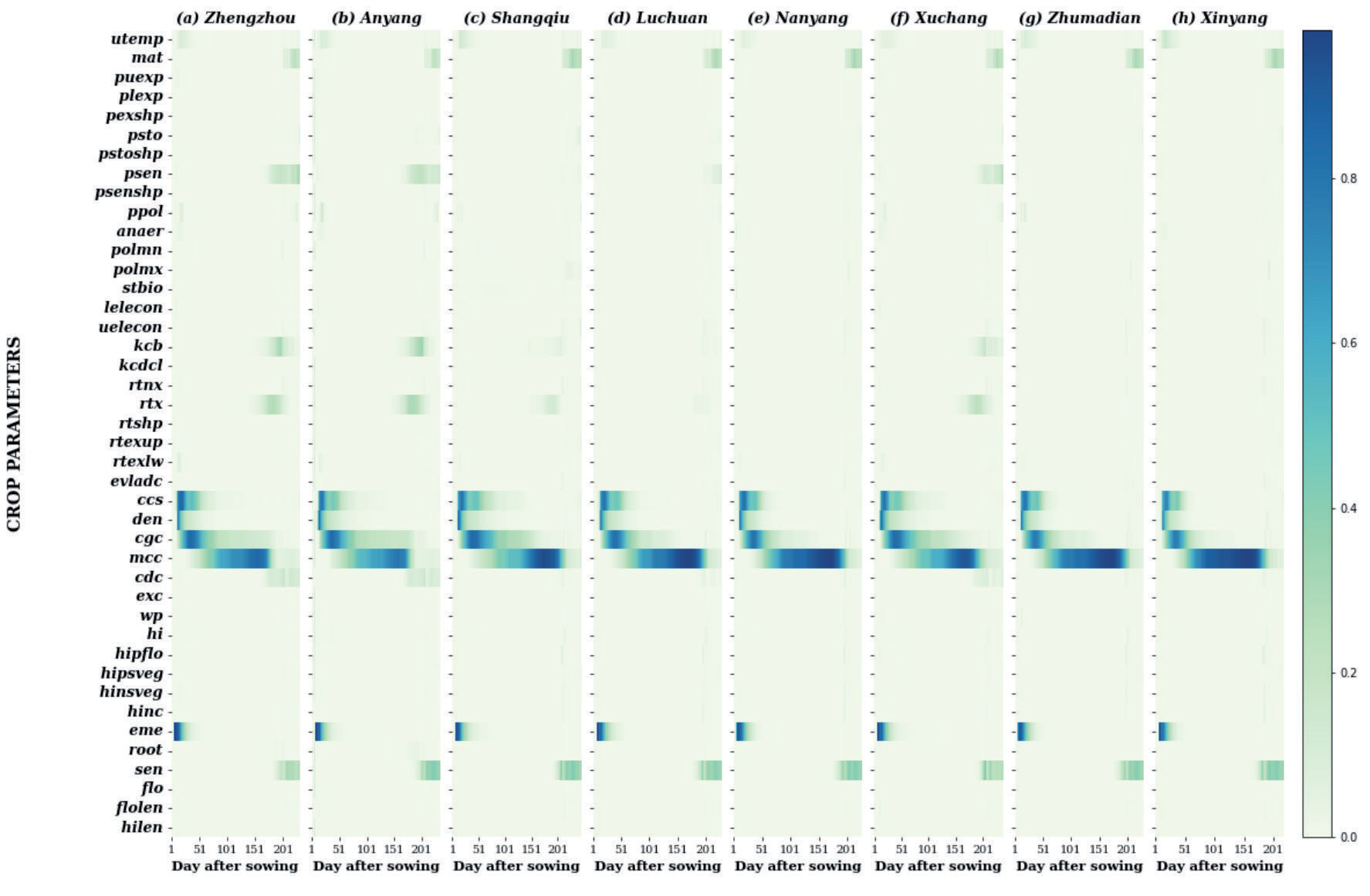
The temporal dynamics of FOSI on CC is shown in Fig. 9. Parameters mcc, cgc, and ccs were the most sensitive parameters. Parameter mcc was more acute in the moderate growth stage of winter wheat (during DAP 70 to 180). Parameters cgc (DAP 17 to 80), den (DAP 12-25), eme (DAP 5 to 28), and ccs (DAP 12 to 50) had high-sensitivity index values in the early growth stage; the sensitivity of parameter sen was mainly manifested in the late phase (after DAP190).
The Temporal Dynamics of TOSI Throughout the Growing Season
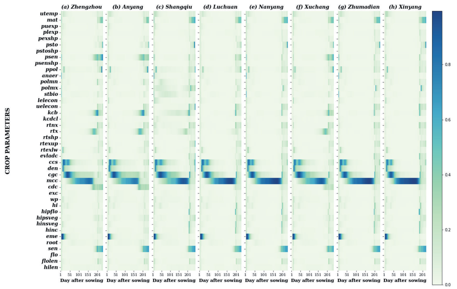
The temporal dynamics of TOSI on CC are shown in Fig. 10. Parameters mcc (after DAP 60) and cgc (after DAP 200 to harvest) were the most sensitive. During the late growth period of winter wheat (about DAP 195 to harvest), the SI of many parameters increased significantly due to the interaction between parameters. The SI parameters kcb, psen, mat, and sen exceeded 0.6. The SI parameters rtx, cdc, and psen were higher in the late stage (about DAP 170 to harvest) in Anyang, Zhengzhou, and Xuchang.
Sum of Sensitivity Index
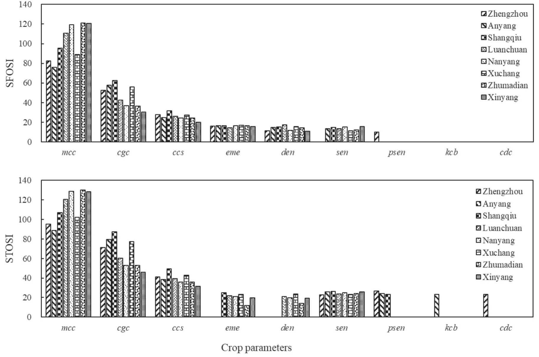
The SFOSI and STOSI on CC are shown in Fig. 11. For the SFOSI, the sensitivity parameters were mcc, cgc, ccs, eme, den, and sen, except for in Zhengzhou where they were mcc, cgc, ccs, eme, den, and psen in Zhengzhou. For STOSI, the sensitivity parameters were different in different study regions. The sum of SI for mcc, cgc, and ccs was the highest, and eme, den, and sen were high in most regions. In some regions (such as Zhengzhou, Anyang, Shangqiu), parameters psen, kcb, and cdc were chosen.
Sensitivity Analysis of Crop Parameters on Yield
The Final Sensitivity Index
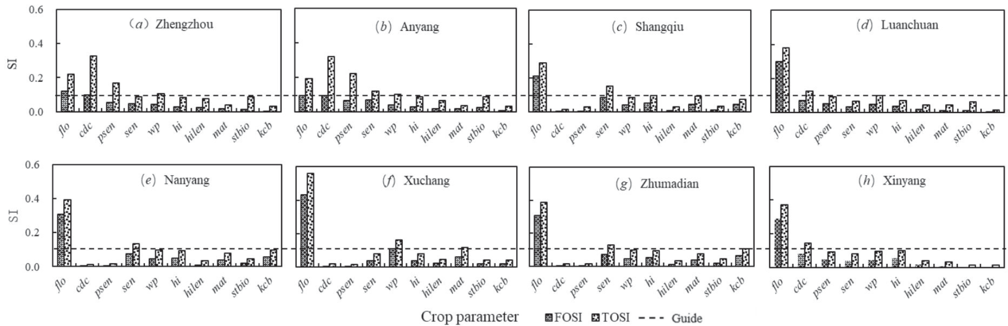
The parameters sensitive to yield are shown in Fig. 12. The sensitive parameters were flo, sen, hi, mat, kcb, and wp in Shangqiu, Nanyang, Xuchang, and Zhumadian, and flo, cdc, and psen in Zhengzhou, Anyang, and Xinyang.
The Temporal Dynamics of FOSI Throughout the Growing Season
The temporal dynamics of FOSI on yield are shown in Fig. 13. From the Figure, there are fewer sensitive parameters to yield, and the selection of sensitive parameters varied significantly in the last 50 days of the winter wheat growth cycle. Parameter flo was the most sensitive, followed by parameters wp and hi; other parameters can be ignored.
The Temporal Dynamics of TOSI Throughout the Growing Season
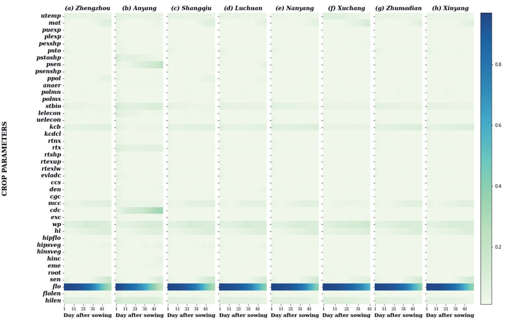
This paragraph discusses the impact of TOSI (temporal dynamics of time series relative importance) on crop yield, using two Figuress (See Fig. 13 and 14) to illustrate the results. In terms of parameter selection, the results for FOSI and TOSI were consistent, but the TOSI values were higher. The parameter flo had the highest SI value, with an average value above 0.6, followed by wp. Additionally, the parameters cdc and psen had a greater impact on crop yield in Anyang and Zhengzhou compared to the other six regions. On the other hand, kcb and hi had a greater impact on crop yield in the other six regions compared to Anyang and Zhengzhou.
Sum of the Sensitivity Index
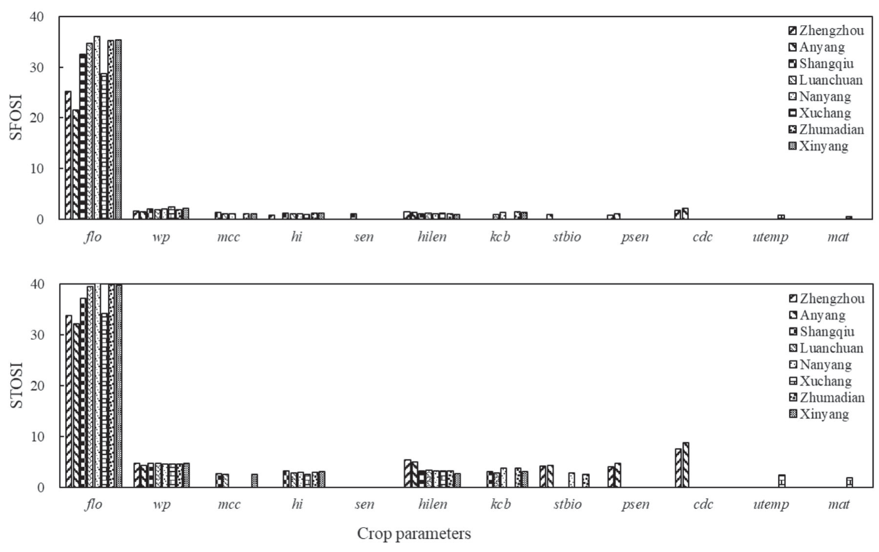
The results of SFOSI and STOSI for yield are presented in Fig. 15. The parameter flo was found to be the most sensitive with SFOSI values exceeding 20 and STOSI values exceeding 30. It should be noted that the selection of sensitivity parameters may vary significantly in different regions due to varying climatic factors. Among the parameters considered, wp and hilen had the highest sum of SI values, while the other parameters exhibited considerable variation.
Discussion
Selection of Sensitivity Index Values
Sensitivity analysis methods include the LSA and GSA methods [2, 14]. The LSA method, by exclusively focusing on the influence of individual parameters on the model’s output, often diminishes the importance of critical elements, primarily due to the neglect of interactions among parameters, ultimately resulting in less-than-optimal outcomes for localized models [31]. The EFAST is the most commonly used GSA method. In this research, we conducted a comprehensive sensitivity analysis of crop parameters within the AquaCrop model across varying regions and meteorological conditions. This analysis was executed using the EFAST method, encompassing both first-order and total-order analyses. Biomass and CC are crucial parameters for winter wheat growth [44] and are commonly used in agricultural model data assimilation, where critical parameters are adjusted to enhance model performance. Among all output variables of crop models, yield is the most critical and commonly used in parameter sensitivity analysis studies [45]. In this model, the output parameters selected were biomass, crop canopy cover (CC), and yield. The sensitivity of the 42 crop parameters was evaluated using both first-order and total-order sensitivity analysis methods. During the simulation of the AquaCrop model, meteorological data, including rainfall, temperature, evapotranspiration, etc., was obtained from local weather station data
This study analyzed 42 parameters, due to a large number of parameters, it is not possible to calibrate all parameters during model localization, and highly sensitive parameters were selected. Those with a low SI can either be set as fixed values or use the reference values provided by the model during model calibration. The final SI selection is based on the FOSI>0.05 and the TOSI>0.1[43]. According to the required reference range for the index values, the final SI value indicates the influence of crop parameters on the output variables. There are six parameters sensitive to biomass (See Fig. 4), including wp, stbio, rtx, mcc, kcb and psen. There are ten parameters sensitive to CC (See Fig. 8), including sen, mat, mcc, uelecon, ppol, rtexup, ccs, psen, cdc, and psto. There are ten parameters sensitive to yield (See Fig. 11), including flo, cdc, psen, sen, wp, hi, hilen, mat, stbio and kcb. However, these indices are not chosen based on the criteria of index selection for each region, but rather a combination of the indices of eight regions.
Fig. 13.
First-order sensitivity indices for a time series on winter wheat yield throughout the growing season.
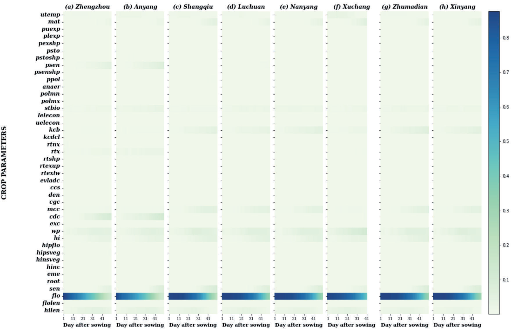
Fig. 14.
Total-order sensitivity indices for a time series on winter wheat yield throughout the growing season.
The final SI value represents the effect of crop parameters on the output variable on the last day but cannot reveal the impact throughout the growth period. However, in the process of simulating crop growth, the influence of parameters on target variables often runs through one or more growth periods. Some parameters – such as cgc, mcc, and eme in the biomass sensitivity analysis, and mcc, cgc, ccs, and den in the CC sensitivity analysis – play essential roles in a particular growth stage of winter wheat but have little impact on the final result. This implies that the sensitivity of the parameters is not constant, but varies with the crop development and the environmental conditions. Therefore, it is necessary to conduct a dynamic sensitivity analysis of crop model parameters to capture the temporal variation of their effects on the model outputs.
The crop model is a process-oriented simulation model that relies on multiple parameters [46]. The sensitivity of the crop parameters varies depending on the region, climate, and crop type. For example, the parameter wp, which represents water productivity, is more sensitive in arid and semi-arid regions than in humid regions, where water stress is less likely to occur. Similarly, the parameter sen, which represents the leaf senescence rate, is more sensitive for crops with longer growing seasons than for crops with shorter growing seasons, where leaf aging is less pronounced. Accurate parameter calibration is crucial for achieving precise simulation results of the crop growth process [36]. It is important to conduct sensitivity analysis throughout the growing season to understand how the model is structured and how the parameters interact with each other over time. Wang et al. [34] pointed out that for dynamic models, the time series dynamics analysis must be considered, and accurate calibration of process variables will improve the accuracy of model simulations. Fig. 5-6 (biomass), Fig. 9-10 (CC), and Fig. 13-14 (yield) show the dynamic changes in the parameter sensitivity values in the whole growth period of winter wheat. It can be found from the Figure that some important parameters (e.g., stbio, kcb, and wp in the biomass sensitivity analysis; mcc, cgc, eme, ccs, and sen in the CC sensitivity analysis; and flo in the yield sensitivity analysis) are not affected by environmental changes in a particular growth stage. However, some other parameters (e.g., eme, cgc, ccs and den in the biomass sensitivity analysis; cgc, eme, and rtx in the CC sensitivity analysis) show significant fluctuations in their sensitivity values over time, indicating that they are sensitive to the environmental conditions and the crop development stages.
Sum of the Sensitivity Index
Fig. 7, 11 and 15 present the sum of the sensitivity index values for biomass, CC, and yield, respectively. The parameters affecting biomass formation are stbio and wp, which have the highest sensitivity values according to both SFOSI and STOSI. The sensitivity order of other parameters (mcc, kcb, eme, and cgc) varies in different regions, indicating that they are influenced by environmental conditions. This conclusion is consistent with Vanuytrecht et al. [47]. The parameters affecting CC are mcc, cgc, and ccs, and this result is consistent with Xing et al. [14]. The sensitivity indices of these parameters differ in different regions, but the ranking remains the same, suggesting that meteorological conditions do not alter their relative importance. The parameters affecting yield are flo, wp, and hilen, which have the highest sensitivity values in most regions. The sensitivity of other parameters, such as mcc and hi, depends on meteorological conditions.
In summary, we can choose ten parameters for the local calibration of the AquaCrop model, they are stbio, wp, mcc, kcb, eme, cgc, flo, ccs, den, and sen. Previous studies have also identified some of the most sensitive parameters of the AquaCrop model for different crops and regions. Zhu [48] conducted a localized calibration of the ten most sensitive parameters, including kcb, hi, wp, cgc, mcc, and others, for maize in the five major maize-production areas of China, which largely matches the results of this study. Rosa et al. [9] conducted a sensitivity analysis of AquaCrop model parameters for wheat in the Campos Gerais region and ranked the parameters, with the top six being HI0 (referred to as hi in this study), WP*(wp), KcTRx(kcb), CCx(mcc), CDC(cdc), and stbio. They also emphasized the importance of water and nutrient management, as well as field management. Orlova et al. [49] provided a set of parameters for model calibration in the AquaCrop model data assimilation, including Maturity(mat), CDC(cdc), CGC(cgc), Flowering(flo), Kcb(kcb), Emergence(eme), Senescence(sen), CCx(mcc), and others.
This study focused on examining how changes in meteorological conditions affect the sensitivity of crop parameters related to biomass, crop canopy coverage, and yield in Henan. However, other factors, such as field irrigation and soil, were not taken into account. Therefore, future research will involve conducting further analysis of the data, broadening the scope of the study, and considering a wider range of factors that may influence crop growth and yield.
This study investigates the impact of meteorological conditions (temperature, precipitation, and sunshine) on the sensitivity of crop parameters, including biomass, CC, and yield, in Henan, a key agricultural province in China. However, it does not account for other influential factors on crop growth and yield, such as field irrigation, soil properties, fertilizer application, crop variety, and field management. Future research will extend this analysis, employing advanced methods like model calibration and verification of crop model parameters. Additionally, it will expand the scope to encompass a broader range of factors affecting crop growth and yield, including crop variety, soil properties, fertilizer application, and field management. These factors, varying spatially and temporally, necessitate extensive data collection and integration.
Conclusions
In this study, 42 crop parameters were selected for performing global sensitivity analysis using the AquaCrop model for biomass, CC, and yield and the EFAST method. Eight regions were part of the study, including Zhengzhou in the Henan Province. The main conclusions were as follows:
(1) For biomass, crop parameter sensitivity is not significantly affected by meteorological conditions, and the most sensitive parameters were stbio, wp, mcc, kcb, eme, and cgc, respectively.
(2) For canopy cover, parameters mcc, cgc, and ccs were the most sensitive; the parameters den and eme were sensitive in the early growth stage of winter wheat; and sen and psen were sensitive in the late stage.
(3) For yield, the parameter flo was the most sensitive; the sensitivity of other parameters varied in different regions depending on climate.
In summary, based on the previously analyzed sensitivity index values for biomass, canopy cover, and yield, the top ten parameters requiring calibration for the AquaCrop model in the Henan region are: stbio, wp, mcc, kcb, eme, ccs, cgc, flo, den and sen.