

Introduction
According to data from the International Energy Agency, China’s carbon emissions reached 9.893 billion tons in 2021 [1]. These large-scale carbon emissions also significantly hindered China’s high-quality development. China has proposed the goal of achieving a carbon peak by 2030 and carbon neutrality by 2060.
China has implemented a new development strategy called “Dual Circulation,” which emphasizes the importance of domestic circulation as the main driver while also promoting the mutually beneficial interaction between domestic and international markets. This strategy aims to facilitate high-quality economic development. Foreign direct investment (FDI) is an essential part of the dual circulation strategy, providing Chinese enterprises with a significant amount of capital, technology, and resources. It serves as a powerful driving force for China’s economic growth. FDI is also a significant component of China’s “Bringing in” strategy, which aims to attract foreign investment, introduce advanced management experience and green technology, infuse new energy into the national economy, and facilitate the optimization and upgrading of the industrial structure. However, it also involves the transfer of high-pollution industries from developed countries, leading to an increase in carbon emissions and environmental degradation. Therefore, foreign direct investment has a specific impact on carbon emissions, but this impact might be nonlinear.
Zhejiang Province is an outward-looking and economically well-developed coastal province in the southeast of China. Zhejiang is a pioneer in China’s reform and opening up. Most of the area is covered by mountains and water, the arable lands are few in Zhejiang. Consequently, Zhejiang’s commercial sectors are highly developed. Since China joined the World Trade Organization in 2001, Zhejiang Province has attracted a large amount of foreign capital. As a result, its economic development and foreign direct investment have consistently ranked among the highest in the country for many years. In 2021, the per capita income of Zhejiang was 113,839 yuan. The urban and rural residents were ranked first among all provinces in China for 21 consecutive years. Moreover, Zhejiang Province has been designated as a demonstration zone for high-quality development and common prosperity. At the same time, FDI not only further stimulates the economy’s vitality, but it also continuously increases energy consumption. The fast growth of the economy leads to a rapid rise in carbon emissions. Zhejiang is one of the most core provinces in the spatial correlation network of carbon emissions in China [2]. The research on carbon emissions in Zhejiang Province can provide some helpful suggestions for other similar regions.
Under the guidance of the “Two Mountains Theory”, Zhejiang’s low-carbon transition is at the forefront of the country. However, the task of achieving carbon peak and carbon neutrality remains very arduous. Under the guidance of the “Action Plan for Carbon Peak by 2030” [3] formulated by the State Council, Zhejiang Province, recognized as a “common prosperity demonstration zone” in the country, has taken the initiative to propose the first provincial-level dual-carbon action plan. Finding a dynamic balance between economic development and environmental protection is a crucial objective for Zhejiang’s high-quality development.
Literature Review
There is a significant disagreement among scholars regarding the impact of FDI on carbon emissions. The main theoretical hypotheses are as follows. The “Pollution Haven” theory, proposed by Copeland and Taylor, argues that developed countries will transfer their high -pollution, low-added-value industries to developing countries through investment, thereby increasing the carbon emissions of the developing country [4]. The “Pollution Halo” theory, proposed by Birdsall and Wheeler, argues that developed countries not only provide development funds to developing countries through FDI but also bring advanced production science, technology and management experience. This changes the overall production concept of local enterprises, improves production efficiency, and reduces carbon emissions [5]. In addition to the two theories mentioned above, the environmental Kuznets theory proposed by Grossman and Krueger argues that pollution will initially increase with economic development. However, once the economy reaches a certain level of development, pollution will subsequently decrease [6]. The empirical analysis results for the aforementioned theories are also inconsistent. Tran utilized the co -integrating nonlinear ARDL model to examine the correlation between FDI and carbon emissions in 62 emerging economies. The study revealed that the relationship between FDI and environmental pollution followed an inverted U-shaped pattern, which is in line with the environmental Kuznets theory [7]. Hou conducted research on FDI and carbon emissions in the eastern, central, and western regions of China. The study found that FDI has a positive impact on China’s overall carbon emissions [8]. Omri studied the panel data of Latin American countries from 1990 to 2011 and found a positive correlation between FDI and carbon emissions [9]. Han-Sol Lee analyzed the panel data from BRICS countries between 2003 and 2017 and confirmed the existence of the “Pollution Haven” hypothesis [10]. However, Hao’s research came to the opposite conclusion. Hao constructed a two-equation model adapted from Halkos and Paizanos to assess the impact of carbon emissions. The final result indicated that FDI could actually help to inhibit the increase of carbon emissions, thus supporting the “Pollution Halo” theory [11]. Similarly, Perkins used a dynamic programming model to study the panel data from 114 countries and also found a negative correlation between the increase in FDI and carbon emissions [12]. Sitthivanh studied nine ASEAN countries and found that FDI not only promotes economic growth and development in ASEAN countries but also helps improve the environmental quality of the region [13]. Song used the two-tier stochastic frontier model to study the panel data of 30 provinces in China from 2007 to 2018. The study found that the promoting effects of FDI are greater than the inhibiting effects in most regions [14]. Yang utilized a threshold regression model to perform an empirical analysis on 30 provinces in China. The study revealed an “inverted U-shaped” relationship between FDI and carbon emissions [15]. Khan utilized the panel co-integration method and panel vector error correction methods to study 108 developing countries and also found evidence supporting the validity of the environmental Kuznets theory in developing countries [16]. Further analysis of the literature found that there was regional heterogeneity in the impact of FDI on carbon emissions. Zhang and Li utilized panel data from 2009 to 2017 to conduct an empirical study on the influence of foreign direct investment (FDI) on carbon emissions in the eastern, central, and western regions of China using panel regression methods. The results showed that FDI in the eastern and central regions all had a carbon emission reduction effect. However, FDI in the western regions had a promotion effect [17]. Arif studied panel data from 45 developed countries and 78 developing countries between 1996 and 2018. He found that the impact of FDI on local areas would vary depending on the local economic conditions [18].
According to the above citations, FDI has a varied impact on carbon emissions. This variation could be attributed to different regions, data sources, or research models. However, it also indicates that the relationship between FDI and carbon emissions is not necessarily linear. There may be nonlinear and structural changes between these two factors. Existing empirical studies primarily utilize linear econometric models to examine the impact of FDI on carbon emissions [19]. However, these models fail to account for the dynamic changes within the system that include FDI and carbon emissions. In recent studies, Pazienza included a quadratic term of FDI to examine whether the correlation between carbon emissions and FDI follows a “U”-shaped pattern [20]. Sarkodie further introduced a cubic term of FDI to study the non-linear relationship between the two variables. Although some scholars have gradually adopted non-linear models for research, their studies have primarily focused on global or national levels. They have not taken into account the varying impacts of FDI on regions at different stages of economic development [21]. The problem of inadequate and uneven economic development among provinces and cities in China remains prominent. If a linear econometric model is directly used to study the relationship between FDI and carbon emissions in China. It will be incorrect if a linear econometric model is directly used to study the relationship between FDI and carbon emissions in China. This paper chooses Zhejiang Province as the research object. As a common prosperity demonstration zone in China, the economic development among counties and cities in Zhejiang Province is relatively balanced. Therefore, studying the relationship between FDI and carbon emissions in Zhejiang Province will reduce the interference caused by regional economic development imbalance. However, in addition to FDI impacting carbon emissions, carbon emissions also affect FDI [22]. Carbon emissions can, to some extent, represent the overall economic scale and level of manufacturing development level. Therefore, in developing countries, a certain level of carbon emissions can stimulate FDI growth and contribute to economic growth and technological development, especially during the early stages when the economy and green technology are not yet fully developed. Therefore, studying the complex nonlinear interaction relationship between carbon emissions and FDI is of great significance for Zhejiang Province in order to achieve a balance between economic development and the ecological environment.
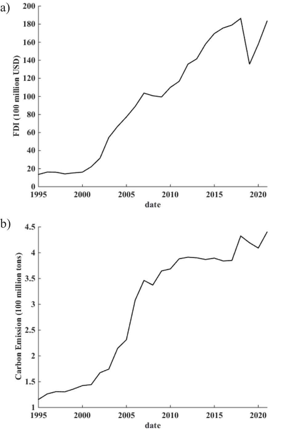
The International Panel on Climate Change (IPCC) pointed out in its “National Greenhouse Gas Inventory Guidelines” released in 2006 [23] that there are six main greenhouse gases that contribute to global warming. Among these gases, carbon dioxide is the most significant [24]. Therefore, this paper uses carbon dioxide emissions as a measure of total carbon emissions. Observing the FDI and carbon emission series of Zhejiang Province from 1997 to 2020 (Fig. 1.), it can be observed that both FDI and carbon emissions in the province generally exhibit fluctuations. Carbon dioxide emissions increased rapidly from 1999 to 2010, and carbon emissions fluctuated upward from 2011 to 2020 with a significantly smaller increase. Overall, FDI increased rapidly from 1997 to 2007. However, due to the impact of the world financial crisis in 2008, Zhejiang’s FDI experienced a short-term decline. It resumed growth in 2010 and reached its highest point in 2018. Due to Sino-US trade frictions in 2019 and 2020, FDI volume dropped sharply. Overall, both the carbon emissions and FDI series of Zhejiang Province showed a clear upward trend, indicating significant non-linearity. Therefore, it can be assumed that under the premise that the social environment and factors remain unchanged, the FDI and carbon emissions of Zhejiang Province constitute an interactive non-linear dynamic system (referred to as FDI-CENLDS).
Hendry believes that describing complex economic problems with a dynamic multivariate nonlinear equation system with certain regularity is difficult. Therefore, establishing a model for solving FDI-CENLDS nonlinear differential dynamic equations is difficult. This paper adopts Hendry’s advocated “data-driven” modeling method, using discrete data from Zhejiang Province between 1995 and 2020 as samples The parameters in the system of differential equation system are estimated using dynamic econometric methods to establish a discrete-type nonlinear dynamic model [25]. This model is transformed into a differential dynamic system model, and numerical solutions are obtained to generate graphical solutions and phase diagrams. This process reveals the possible nonlinear interaction relationship between FDI and carbon emissions in Zhejiang Province, as well as its optimal solution.
Materials and Methods
Assumptions
The basic assumption of the general model of FDI-CENLDS is that as long as the nonlinear dynamic equation is reasonable, all the information regarding the nonlinear behavior characteristics of the relationship between FDI and carbon emissions is contained in the structure and coefficients of the equation. In addition, the study of the FDI-CENLDS nonlinear system requires the following assumptions.
Fig. 1.
a) The values of FDI in Zhejiang Province from 1995 to 2021; b) The values of carbon emission in Zhejiang Province from 1995 to 2021.
Assumption 1: Systematicity. Under the premise of excluding the influence of other possible variables on FDI and carbon emissions, FDI-CENLDS is a whole formed by their mutual nonlinear interaction.
Assumption 2: Non-randomness. There may be random effects in the nonlinear system. If the random effects can reach a balanced state, non-random factors can be ignored. As a two-dimensional system, the trajectory of the system will not be affected by changes in the previous state, initial values, or equilibrium shocks.
Assumption 3: Continuity. FDI-CENLDS is a continuous system, and FDI and carbon emissions are continuous functions of time. They are independent of spatial distribution and are solutions to differential equations.
Assumption 4: Differentiability. It is impossible to directly establish differential equations in empirical analysis. However, if the nonlinear system is considered as a discrete differentiable system, statistical data can be used to establish different equations, regardless of whether the data generation process of the two is stationary or not. These different equations can then be transformed into differential equations.
Materials and Data
The FDI data in this paper comes from the Statistical Yearbook of Zhejiang Province, 1996-2022. Total carbon emissions are measured by carbon dioxide emissions, and data on all types of energy are from the China Energy Statistics Yearbook 1996-2022. The calculation of carbon dioxide emissions is based on the formula provided by the IPCC Guidelines for National Greenhouse Gas Emission Inventories, 2006 edition. Carbon dioxide emissions from Zhejiang Province have been calculated from 1995 to 2021 using formula (1):
CE represents the carbon dioxide emissions of Zhejiang Province. E is the total energy consumption. NCV represents the energy conversion factor, while CEF stands for the carbon emission factor of the energy. The types of energy consumption, along with their energy conversion factors and carbon emission factors, are derived from the IPCC Guidelines for National Greenhouse Gas Emission Inventories (2006 edition), as shown in Table 1.
Theory and Mechanism Analysis
According to the concept of dynamic economic modeling idea [26], there may be various interaction relationships between FDI and carbon emissions in Zhejiang Province, including self-effect, coupling effect, or spillover effect.
In FDI-CENLDS, when there is no transmission mechanism between FDI and CE, both FDI and CE evolve independently according to their own laws. They can either increase or decrease on their own, which is known as the self-effect. The kinetic equation is as follows:
f1 and f2 are the evolution laws of FDI and CE respectively. According to the formula, self-effect is an effect brought by themselves.
When CE and FDI are mutually affected by the other party, it shows as the coupling effect, which is an indirect transmission effect. The interaction between CE and FDI is called the coupling effect. The kinetic equation is as follows:
Table 1.
Energy conversion coefficient NCV and carbon emission coefficient CEF.
g1 and g2 are the coupling effects of FDI and CE from the interaction between FDI and CE.
and when CE and FDI evolve according to their own laws, while also having a certain impact on the other party, forming external benefits, which is the spillover effect. Previous research has shown that FDI has a significant impact on carbon emissions [27]. For instance, Mahadevan found that FDI has no impact on carbon emissions in some countries [28]. Deng found that FDI, whether it is too low or too high, has no impact on carbon emissions [29]. It should be added that FDI has different impacts on different regions [30].
h1 is the spillover effect of FDI for CE; h2 is the spillover effect of CE for FDI.
Model Development and Methodology
In order to study the possible interaction relationships between FDI and CE, based on the basic assumptions, the generalized Lotka-Volterra model is extended to obtain the FDI-CENLDS discrete model that can reflect the possible interaction relationships between FDI and CE.
In model (5), α, β, γ, δ, ε, ζ, η, θ, ι, κ, λ, and ξ are coefficient terms, and μ1 and μ2 are residual terms. If the residual series is stationary, then FDI and CE have a cointegration relationship. If the model has a high explanatory power, indicated by a high R2 value, then the functional relationship can be approximated. In this case, the difference model and the differential model can be transformed into each other. Model (5) is transformed into the general model of FDI-CENLDS:
Model (6) is a nonlinear dynamic system of FDI and CE, known as the FDI-CENLDS model. It represents a system evolution equation with the highest power of two. This model has the following special cases:
(1) When η, θ, ι, κ, λ, and ξ are not significant, FDI and CE are regarded as two independently developing systems with their own evolutionary mechanisms. If γ and δ are greater than 1, it indicates that FDI and CE have a positive feedback mechanism. If γ and δ are less than 1, it indicates that FDI and CE have a negative feedback mechanism. If ε and ζ are greater than 0, it indicates that FDI and CE have an acceleration mechanism. If ε and ζ are less than 0, it indicates that FDI and CE have a deceleration mechanism.
(2) When both η and θ are less than 0, it indicates a competitive relationship between FDI and CE. When both η and θ are greater than 0, it indicates a synergistic effect between FDI and CE, forming a mutually beneficial relationship. When η and θ have different signs, it indicates a predatory relationship between FDI and CE. When one of η and θ is 0 and the other is greater than 0, it indicates a coexistence relationship between FDI and CE.
(3) When ι, κ, λ, and ξ are greater than 0, it indicates a mutual aid relationship between FDI and CE. Conversely, when ι, κ, λ, and ξ are less than 0, it indicates a competitive relationship between FDI and CE. λ and ξ are acceleration coefficients.
Table 2.
Discrete model and statistics of FDI-CENLDS in Zhejiang.
(4) When ε, ζ, η, θ, λ, and ξ are equal to 0, FDI-CENLDS is considered a non-autonomous linear system.
(5) When γ and δ are greater than 1, and α, β, ε, ζ, η, θ, ι, κ, λ, and ξ are all greater than 0, it indicates that FDI and CE have causal relationships with each other. They mutually promote each other, leading to co-evolution. This is the most ideal relationship.
Results
Based on Fig. 1., the discrete model measurement results of FDI-CENLDS in Zhejiang are obtained by EViews software (Table 2).
It can be seen from Table 2 that when the significance level is 5%, the regression coefficients of the two nonlinear equations in the discrete model (5) are significant. The goodness of fit is high, and the model has a stronger explanatory power. Therefore, the functional relationship can be approximated by the discrete econometric model, and the discrete model can be transformed into a continuous FDI-CENLDS model. The Durbin-Watson (DW) value in the discrete model is approximately 2, indicating that there is no autocorrelation in the residual sequence of the model. It can be considered that the model captures the relevant information in the time series.
The residual terms were further subjected to the ADF smoothness test. The results of the ADF test are shown in Table 3.
It can be seen from Table 3 that the ADF values are all less than the MacKinnon critical value at the 5% level. Therefore, the residual terms μ1 and μ2 residual sequences are stable. There is a stable long-term cointegration relationship between FDI and CE in Model (5). FDI-CENLDS is a cointegration system formed by the interaction between FDI and CE variables.
As Table 2 shows, the discrete model is transformed into a continuous FDI-CENLDS differential dynamic system model:
It can be seen from Model (7) that there are four nonlinear terms in the FDI-CENLDS differential dynamic system model, and it does not include a time variable. Therefore, FDI-CENLDS is an autonomous nonlinear plane dynamic system. Among them, for CE, there is a first-order negative feedback mechanism, the coupling effect with FDI has a negative growth effect, and the spillover effect of FDI has a direct driving effect on CE. For FDI, there is a first-order negative feedback mechanism, and the coupling effect with CE has a positive impact on economic growth. The equation contains CE and CE2 with different signs, so CE can play a role in regulating the speed of FDI. Further analysis shows that when CE is greater than 1.2611, the growth rate of FDI is inhibited, and vice versa. Because both FDI and CE have a first-order negative feedback mechanism, they possess a self-inhibition mechanism. This means that the rate of change will gradually decrease until the system reaches a stable state. The sign of the coupling term in the two equations indicates that the coupling term has a positive impact on the growth of FDI and a negative impact on the growth of CE. However, there is also a positive spillover effect brought from FDI to CE. Therefore, the impact of FDI on CE will vary depending on the size of CE. The partial derivative of the equation with respect to FDI is obtained, that is:
Table 3.
Discrete model and statistics of FDI-CENLDS in Zhejiang.
| DF-equation test | Adj. R2 | F | ADF | MacKinnon critical value (5%) | |
|---|---|---|---|---|---|
| μ1 | ∆u1 = −0.4467 −1.1992u1,t−1 | 0.5880 | 30.9608 | -5.5642 (0.0002) | -3.0049 |
| μ2 | ∆u2 = 0.0063 1.1683− u2,t−1 | 0.4512 | 18.2645 | -4.2737 (0.0033) | -3.0049 |
Let the derivative function (8) be 0. When CE = 4.7941, it can be observed that an increase of FDI will promote the growth of carbon emissions. When CE>4.7941, ∂/∂ FDI<0, indicating that when carbon emissions reach the critical point of 479.41 million tons, FDI will begin to inhibit the growth of carbon emissions.
The velocity divergence of Model (7) is further solved. That is:
According to the Equation (9), CE accelerates the growth of the entire FDI-CENLDS system, while FDI has a decelerating or dissipating effect on the system. The velocity divergence of FDI-CENLDS is controlled by a plane with a positive and negative boundary. For different combinations of CE and FDI, there are varying zero lines. After FDI exceeds a certain threshold, FDI-CENLDS will tend to become an attractor over time. This shows that FDI-CENLDS has the most advantages.
According to the assumption, the structure and coefficients of the equation contain information about the nonlinear behavior characteristic of the relationship between the two. Because Model (7) contains four nonlinear terms, there are strong nonlinear factors, which result in a more complex functional relationship of the model. This complexity leads to high computational complexity in numerical calculations. In the iterative process of solving, errors such as vibration or divergence may occur, even if the approximate numerical solution is not accurate. Therefore, it is better to use numerical methods for analysis.
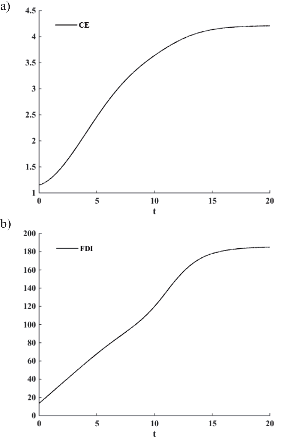
It can be seen from Fig. 2a) and Fig. 2b) that the development of the two shows two-stage characteristics. Both FDI and CE will converge to a stable value after a period of rapid growth, indicating the existence of an equilibrium point between the two.
Fig. 2.
a) The Numerical Analysis of C in FDI-CENLDS; b) The Numerical Analysis of FDI in FDI-CENLDS.
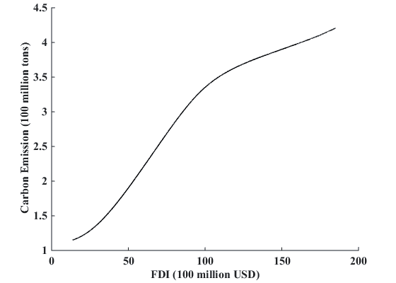
From observing the phase diagram (Fig. 3), it can be seen that the relationship between the two also exhibits a two-stage characteristic. After an initial phase of quasi-linear rapid growth, it enters a state of slow growth. Therefore, the relationship between CE and FDI is not linear, and there are equilibrium points between the two.
By observing the graphical solution and phase diagram of the FDI-CENLDS model, it can be concluded that there is an equilibrium point in the FDI-CENLDS model. The existence of an equilibrium point in the model is a necessary condition for model stability of the model, but it does not guarantee that the equilibrium point will be stable. Therefore, it is necessary to study the stability of the equilibrium point. Since FDI-CENLDS is a continuous and smooth nonlinear system, the system equation can be expanded by Taylor expansion and approximated using first-order or higher-order polynomials. When the system is close to the zero point, the nonlinear term near the zero point has little effect and can be considered a weak nonlinear term. Therefore, the nonlinear function can be approximated as a first-order term near the zero point, and then the nonlinear system can be linearized. Then, according to the linear theory, the stability of the system is studied. The Jacobian matrix is a linearized approximation matrix of the nonlinear system near the equilibrium point. It contains the key information about the system dynamics. In order to find the stable equilibrium point of the system, which is the optimal point (FDI *, CE *), the Jacobian matrix J of Model (7) is established :
Let dCE/dt = 0, dFDI/dt = 0, E1 = (329.8228, 4.4493).
Therefore, the value of the Jacobian matrix in E1 is JE1:
The eigenvalue of JE1 : λ1 = -5.8480<0, λ2= -1.1382<0;
According to the Routh-Hurwitz theorem [31], if the determinant value of the matrix is less than 0, it indicates that the linearization of FDI-CENLDS near this point does not provide sufficient information to determine the stability of the system is stable at this point. Additionally, the signs of the two eigenvalues are different. There are unstable modes in both positive and negative directions near this point. That is, the behavior of the system will deviate from the equilibrium point, indicating that the point is unstable. The determinant of JE1 is greater than 0, and the eigenvalues are of the same sign and less than 0. This indicates that when the system deviates slightly from the equilibrium point, it tends to return to the vicinity of this point. Therefore, E1 is a stable equilibrium point and the equilibrium point is the stagnation point of the FDI-CENLDS dynamic model, so E1 is the optimal point of FDI-CENLDS, represented as (FDI *, CE *) = E1 = (329.8228,4.4493). At this point, FDI and CE will be in a stable state, which is the optimal state of FDI-CENLDS.
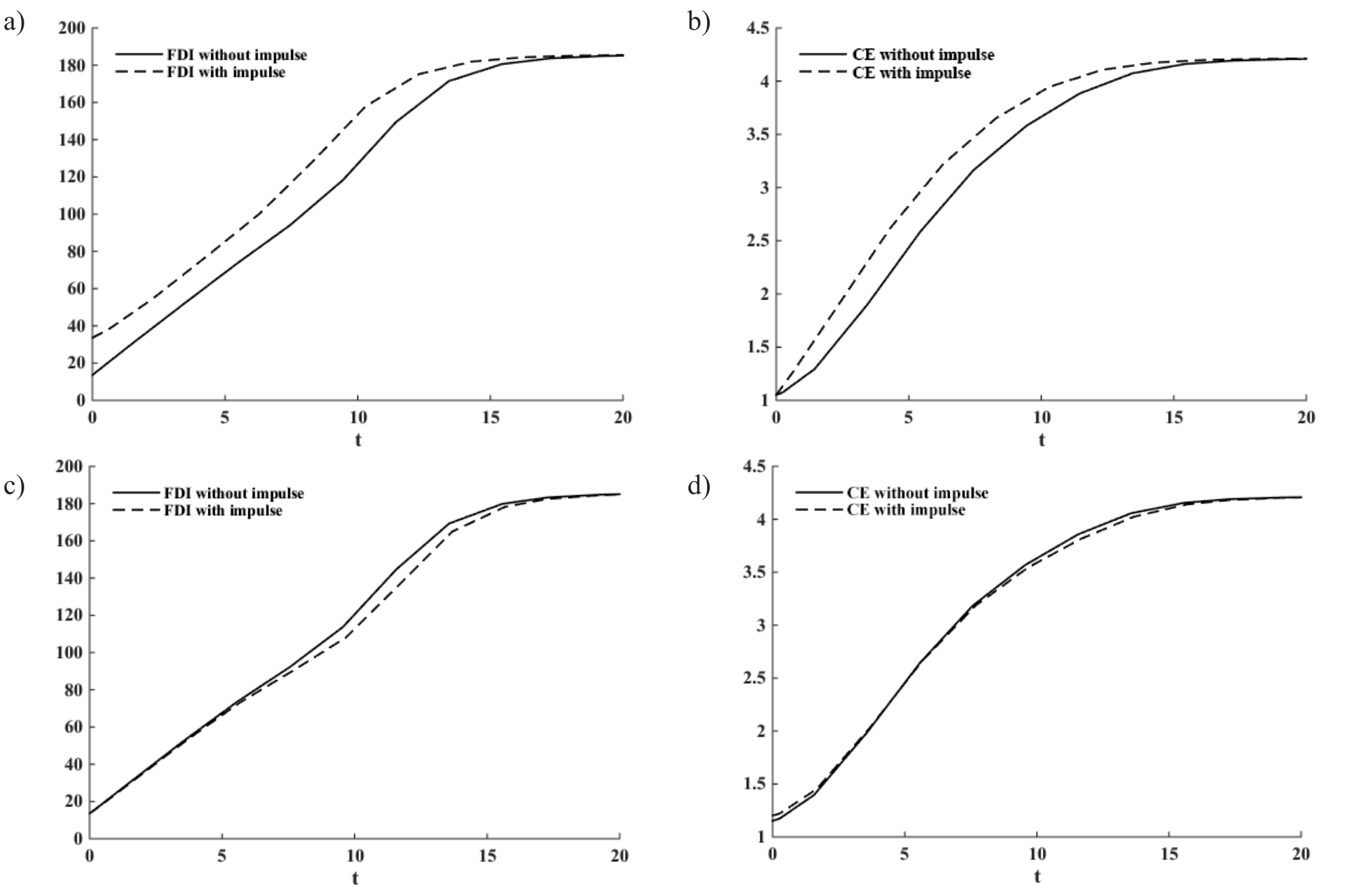
Although FDI-CENLDS may be considered the optimal point of E1, it is important to note that FDI-CENLDS is not a closed system. Instead, it is an open and dynamic system that can be influenced and disrupted by external factors, ultimately affecting its overall stability. Therefore, the pulse experiment is conducted to investigate the detection system’s sensitivity to external shocks.
When a shock of 2 billion USD is applied to the initial value of FDI0 (Fig. 4(a, b)), the FDI-CENLDS system exhibits a specific response. FDI and CE show clear signs of growth acceleration, but ultimately, they will tend to stabilize, indicating that FDI-CENLDS is not sensitive to the impact of FDI0.
Applying a shock of 5 million tons to the initial value CE0 of carbon emission CE (Fig. 4(c, d)), the FDI-CENLDS system exhibits a specific response. Under the shock of 5 million tons of carbon dioxide emissions, the growth rate of FDI has slowed down slightly. However, after a period of development, the impact of the shock has gradually weakened. Under the impact, the growth rate of CE increased significantly. However, the growth rate gradually slowed down, and the impact gradually weakened until it disappeared.
The above initial impact experiment above shows that the FDI-CENLDS system in Zhejiang Province is not very responsive to the impact. When the impact occurs, after a period of development, the intensity of the impact will gradually weaken until it disappears, indicating that the FDI-CENLDS system is stable.
Findings
Analysis of the Mechanism of FDI and Carbon Emissions in Zhejiang Province
By constructing a nonlinear dynamic system of FDI and carbon emissions, it is found that there exists a nonlinear relationship between FDI and carbon emissions. In the FDI-CENLDS model, there is a negative feedback mechanism between carbon emissions and FDI in Zhejiang Province. Carbon emissions and FDI also interact with each other. When carbon emissions are less than 479.41 million tons, an increase in FDI will promote the growth of carbon emissions. However, when carbon emissions exceed 479.41 million tons, the growth of carbon emissions will be inhibited. The rate of change between the two will gradually decrease until it reaches a stable level. Carbon emissions in Zhejiang Province indirectly regulate the growth of FDI. When carbon emissions are less than 1261.1 million tons, an increase in carbon emissions will promote the growth rate of FDI. Conversely, when carbon emissions exceed 1261.1 million tons, the growth rate of FDI will be inhibited. Zhejiang’s carbon emissions in 2021 were 440.16 million tons. This suggests that the recent surge in FDI in Zhejiang has contributed to the rise in carbon emissions, while the increase in carbon emissions has inhibited the growth of FDI. Previous studies have concluded that the technology spillover effect of FDI can significantly reduce carbon emissions [32]. However, the conclusion of this paper is that the increase of FDI promotes the growth of carbon emissions. This indicates that the technological effect of FDI in Zhejiang Province has not fully played its role. Zhejiang Province needs to improve the quality of investment attraction while expanding the scale of FDI, actively introducing high-tech production technology, encouraging foreign capital to enter clean energy fields, and implementing more stringent restrictions on the introduction of FDI. In addition, the current increase in carbon emissions in Zhejiang has inhibited the growth rate of FDI. This shows that although Zhejiang is implementing the two-mountain theory and prioritizing the development of a low-carbon economy, the province still needs to enhance environmental regulations and improve the efficiency of resource utilization.
The Optimal Scale Analysis of FDI and CE in Zhejiang Province
By studying the zero point of FDI-CENLDS and conducting a sensitivity analysis of the zero point, the optimal point (FDI*, CE*) of FDI-CENLDS is obtained. Further research on the stability of the system reveals that the system is not sensitive to the initial pulse. The optimal point is also the stable point. Therefore, the optimal FDI* of Zhejiang Province is 32.98228 billion USD, and the optimal carbon emissions CE* are 4.4493 million tons. In 2021, Zhejiang’s FDI was 183.3970 billion USD, which is still significantly below the optimal scale of FDI of 329.8228 billion USD. Professor Li proposed that from 2021 to 2025, the average annual growth rate of China’s FDI should reach 5% in an optimistic scenario [33]. If the average annual growth rate of FDI is 5%, Zhejiang’s FDI will be 222.4376 billion USD in 2025. FDI still has a large room for further development. Therefore, Zhejiang should increase its foreign direct investment inflows. In 2021, Zhejiang’s carbon emissions will be 440.16 million tons, which exceeds the optimal scale of carbon emissions by 444.93 million tons. Although the current carbon emissions in Zhejiang Province have not yet exceeded the optimal scale, they are very close. This shows that Zhejiang Province, as the birthplace of the “Two Mountains Theory” has achieved significant results in low-carbon development and green transformation in the early stage. Additionally, carbon emission control is more favorable in the province. However, Zhejiang Province should continue to maintain the pace of energy conservation and emission reduction. It should also strengthen the environmental supervision of foreign investment projects while vigorously attracting FDI. It also should encourage foreign direct investors to establish green supply chain cooperation with local Chinese enterprises. This will help to jointly promote the sustainable use of resources and energy, facilitate technological exchanges and cooperation among enterprises, and collectively seek solutions to reduce carbon emissions. Ultimately, this will ensure that FDI and carbon emissions develop to the optimal scale.
Conclusions
This study set out to analyze the relationship between FDI and carbon emissions and the optimal scale of FDI and CE. The analysis revealed that the relation between FDI and carbon emissions is complex and nonlinear. The optimal scale for FDI and carbon emissions is 183.3970 billion USD and 444.93 million tons respectively.
This study has enriched the research about the influential factors of carbon emissions and provided a deeper insight into the relationship between FDI and carbon emissions. Moreover, This paper verifies the existence of a nonlinear relationship between CE and FDI. This article confirmed the existence of the optimal scale for FDI and carbon emissions.
The above results suggest that the government should increase the promotion of FDI and pay more attention to the quality of FDI. The government should strengthen environmental supervision of foreign investment projects while vigorously introducing FDI. The insights gained from this study may be of assistance in keeping a balance between economic development and the ecological environment.
However, due to my limited knowledge, energy, and access to data resources, the research and analysis of theory are not comprehensive enough. It should also consider factors such as exchange rates and policies.

