

Introduction
Air pollution is a worldwide concern due to its hazardous effects on human health [1, 2]. Tracing and positioning the source of airborne pollutants is necessary and crucial for both pollution control and management and, subsequently, improving air quality and ensuring human health [3]. Conventional air pollution monitoring facilities are mainly fixed monitoring stations [4]. In the recent decade, vehicle-mounted monitoring stations and wireless sensors for airborne pollutants have attracted the attention of researchers and administrators [5, 6], who can both monitor air quality and estimate the geographical location of pollution sources based on the site of the stations and the concentration gradients of pollutants. Chiang et al. established a vehicle-based monitoring system installed on vehicles traveling on streets to collect real-time data, recording PM2.5 concentrations in areas surrounding people’s residences [7]. Li et al. developed an air pollution tracking model using a wireless sensor system (WSS) that utilizes sensor nodes and a fixed system to track air quality [8]. In addition, Bhatti et al. studied the current status of particulate matter of air pollution (PM2.5) in the city of Lahore, Pakistan, analyzed its influencing factors and predicted the future PM2.5 concentrations using the SARIMA model [9]. However, it is urgent to develop a more effective and practical monitoring system that can realize the traceability and location of pollution sources [10].
In recent years, remote sensing technology has gradually been applied to various phenomena and fields, such as the weather, geology, disaster prediction, and urban planning [11]. Unmanned aerial vehicles (UAVs) have been widely adopted in various fields, such as military [12], earth sciences [13, 14], natural disaster warning [15], and video surveillance [16, 17], due to their flexibility and mobility[18, 19]. The application of UAVs equipped with gas sensors for air pollutant monitoring is snowballing [20, 21]. For instance, Li et al. used a lightweight UAV with a tethered balloon platform to investigate the three-dimensional distribution of ozone and particulate matter (PM2.5) concentrations in the lower troposphere at 1,000 meters at a localized coastal area in Shanghai, China [22].
To date, few researchers have used UAVs to trace air pollution sources. Yunagicela-naula et al. utilized unmanned aerial vehicles (UAVs) equipped with sensors to detect pollutant concentrations for source tracing in simulated high-turbulence pollution environments [23]. Castro et al. designed a UAV system for locating gas sources in windless indoor environments [24]. Le et al. focused on using single and multiple drones to detect pollution sources in industrial parks [25]. The methods of tracing pollution sources can mainly be divided into two types: source traceability in a probabilistic context and source traceability based on the concentration gradient. Most probabilistic source tracing methods are based on Bayesian inference and its optimization methods, mainly relying on electronic nose sensors to identify the pollutants but not actively tracing the source [26, 27] due to their design and functionality. The primary role of electronic nose sensors is to detect and analyze the gas composition in the environment rather than actively locating the source of pollution. The data provided by the sensors is used as input for establishing probability models and conducting Bayesian inference, helping researchers understand how pollutants diffuse and the possible direction or region they may originate from. Gradient-based methods can more directly locate the source by relying on the signal emitted by the source or the variation of physical characteristics with distance. Thus, it is essential to conduct the pollution source tracing based on the concentration gradients, which can actively implement the task [28]. Yungaicela-Naula et al. proposed an algorithm for locating air pollution sources using Unmanned Aerial Vehicles (UAVs) [29], and the algorithm combined a gradient-based search with a probabilistic approach to locate pollution sources. The design of the gradient-based search component was based on a simulated annealing metaheuristic and allowed tracking of the pollutant plume.
Source localization methods combined with swarm intelligence optimization algorithms are the most commonly used methods for active source tracking in the most current research. Saadaoui et al. proposed a probabilistic search strategy based on the Local Particle Swarm Optimization (LoPSO) method [30]. In this approach, each particle learns from the unique best experience generated by the new search strategy to optimize the unmanned aerial vehicle’s search path. The optimization strategy enhances the collaborative search of UAVs, improves the efficiency of earthquake source detection, and reduces the overall search time. Jiang et al. proposed a new algorithm called Fuzzy Control Traceability (FCT) to track the odor plume [31]. The algorithm combined the characteristics of UAVs and fuzzy control to design a controller based on the actual environment of UAVs. The fuzzy controller fuzzily processed the input gas concentration information, established fuzzy control rules, and outputted the turning angle and movement length according to the rules, thus achieving intelligent tracking of the odor plume by the UAV. Liu et al. addressed the problems of lower UAV search efficiency due to unplanned search routes, possible local extrema and internal collisions, the inability to locate the odor source quickly, etc. [32].
The Particle Swarm Optimization (PSO) algorithm possesses simplicity, fast convergence, robustness, distributed collaboration, and adaptability characteristics. It can simulate collective behavior, support parallel computing, and effectively avoid local optima. Gunawardena et al. presented a method for locating a pollutant source in complex urban environments using the particle swarm optimization (PSO) algorithm. This method applies PSO to unmanned aerial vehicles (UAVs) and uses the QUIC model to simulate pollution plumes in urban environments [33]. Nayeem et al. analyzed various inertia-weight PSO algorithms for enhancing particle diversity and proposed an adaptive time-varying inertia-weight parameter for their previously proposed nPSO algorithm for UAV path planning, comparing its performance with other inertia-weight strategies [34]. Therefore, this paper proposed an improved particle swarm optimization (IPSO) algorithm that combines PSO with a sawtooth algorithm to pre-plan the search routes and improve the efficiency of UAV search plumes.
UAVs with environmental sensors can be highly efficient in collecting environmental information and analyzing the time-dependent variation in pollutant concentrations. However, there are still some challenges in using UAVs for tracing air pollution sources, such as detecting large-scale air pollution at the limited flying time of UAVs and measuring the dynamic change of atmospheric pollutant concentration using a global static optimal allocation of traceability. Thus, this study aims to establish an effective Multi-UAV Cluster Traceability Distributed (MCTD) control structure to solve the above-mentioned problems. Meanwhile, a dynamic suppression psychological (DSP) algorithm for multi-UAV inspired by the social impact theory was proposed. Finally, a high success rate of source tracing for target pollutants (over 80%) was achieved. Unfortunately, only stationary sources of pollution were considered in this paper, not moving sources. Based on the research on the traceability of stationary pollution sources, we will think about how to apply the algorithms proposed in this paper to the traceability of moving sources in the future.
Materials and Methods
Multi-UAV Cluster Traceability Distributed (MCTD) Control Structure
The MCTD control structure is mainly composed of a UAV ground control station and a set of UAVs, as shown in Fig. 1a) and 1b). Fig. 1c) shows the specific communication process. Moreover, the innovation of the MCTD control structure is that UAVs in the same group can exchange monitoring messages of air pollutant concentrations from other groups of UAVs through the ground control station. This is crucial for determining the highest point for measuring the global concentration of the pollutant.
Fig. 1.
The design of the Multi-UAV Cluster Traceability Distributed (MCTD) control structure created in this study.
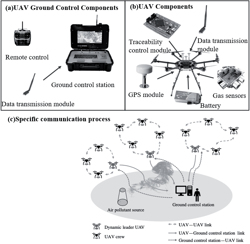
The ground control station for unmanned aerial vehicles (UAVs) consists of a remote controller and a data transmission module, as depicted in Fig. 1a). It is responsible for remote control and the sending/ receiving of data. Each UAV is equipped with a tracking control module, a data transmission module, a GPS module, a battery, and a gas sensor, as depicted in Fig. 1b). These modules work together to collect information such as air pollutant concentrations, environmental parameters, and weather conditions. The ground control station establishes a bidirectional communication link with the UAVs to ensure real-time information exchange. Firstly, based on the nature and requirements of the mission, the ground control station groups the UAV fleet and assigns a dynamic leader of the UAV from a distributed control structure to each group. The dynamic leader of the UAV, acting as the leader of the group, collects and consolidates environmental information from the UAVs within the group through the data transmission module. It then transmits this information to the ground control station, thus avoiding redundant information transmission and reducing the information processing burden on the ground control station. Secondly, the dynamic leader UAV can also send cooperative search tasks and other information to the UAV fleet through the data transmission module, as shown by the lines of UAV-Ground control station link and Ground control station-UAV link in Fig. 1c). Each group operates independently under the guidance of the dynamic leader UAV, and other UAVs within the group can receive data on air pollutant concentrations and external environmental information from the dynamic leader UAV. In applying the Particle Swarm Optimization (PSO) algorithm, each UAV is considered an agent (particle) in the algorithm. The UAVs within the same group exchange information through wireless communication to search for the optimal solution within the search area, such as the location of pollutant sources or the best flight path, as illustrated by the lines of UAV-UAV link in Fig. 1c). This approach allows the UAV fleet to intelligently adapt to environmental changes and optimize search behavior.
Dynamic Suppression Psychological Algorithm of Multi-UAV
The basic PSO (particle swarm optimization) algorithm is based on bird foraging and simulates a bionic optimization algorithm for social behavior between groups in nature. Each particle has its position and velocity and an optimal value determined by the optimization function. Each particle knows its optimal position and the optimal position of the whole group, and in each iteration, the particle is updated by tracking the two optimal positions until the optimal solution is found. The particles update their position and velocity by the following Equation:
where w is the inertia weight, c1 and c2 are the “cognitive learning factor” and “social learning factor”, respectively, which are used to adjust the weight of the particle’s own experience and the group’s social experience in its movement, β1 and β2 are random numbers from 0 to 1, Pbest is the individual historical optimal position, and Gbest is the global optimal position.
The first part of Equation (1) is the velocity of the particle in its last iteration; the second part, called the “cognitive” part, represents the effect of the particle’s state on its velocity; and the third part, the “social” part, represents the sharing of information between particles and reflects the effect of other particles in the population on a single body.
The basic PSO algorithm is prone to falling into local extrema for functions with multiple local extrema. It often fails to obtain accurate results due to the lack of cooperation with sophisticated search methods. Although the PSO algorithm has been applied and improved in existing research on pollution source location [30, 32], it still has shortcomings. Therefore, this paper innovatively proposed a multi-UAV dynamic suppression psychological (DSP) algorithm inspired by social influence theory.
This paper discusses the theory of social impact, which is a widely observed social psychological phenomenon. It describes how individuals’ behavior and attitudes tend to align with prevailing social trends under the influence of social pressures. This phenomenon includes obedience, conformity, social facilitation, social loafing, group polarization, and collective thinking.
The dynamic suppression psychological (DSP) algorithm of multi-UAV is inspired by the social impact theory based on the basic PSO algorithms [35]. This theory considers the social influence within a given social environment, which depends on factors such as quantity, intensity, and immediacy. In the process of tracking air pollution, the interactions among multiple UAVs resemble interactions within a social group. The concept of dynamic suppression is reflected in multi-UAV tasks, where each UAV’s actions are influenced by its own state and the states of other UAVs. When a task performer falls behind other team members, they are suppressed to take proactive measures and catch up with the team’s progress.
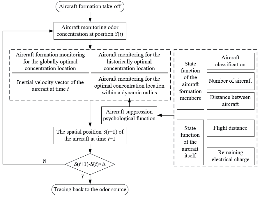
Compared with the traditional PSO algorithm, this paper introduced the maximum contaminant 3D spatial location within the dynamic radius of the UAV in the Multi-UAV Cluster Tracking Distributed (MCTD) control structure, which fits the actual UAV application scenario and can improve the algorithm performance. The analysis is as follows: Firstly, each dynamic UAV group leader is equivalent to a small ground control station, which compares the concentration of pollutants detected by the UAV members (crew) in the group to obtain the maximum concentration in the dynamic range, reducing the amount of data processing by the ground control station. Secondly, based on the traditional PSO algorithm, after introducing the 3D spatial location of the maximum pollutant in the dynamic range, each UAV in the group will have a certain probability of flying to the location of the maximum pollutant in the dynamic range, which can, to a certain extent, improve the potential of circumventing the possibility of falling into the local optimum, thus improving its success rate of tracing the source of pollution. The DSP algorithm is associated with the function of suppression psychology and is primarily influenced by the status functions of other UAVs within the group and the UAV’s own status function. As the psychological suppression value of UAVs increases, the dynamic radius of UAVs can expand, enriching the environmental information within the dynamic radius. These factors can enhance the traceability of atmospheric pollution sources. Fig. 2 shows the overall flow of the collaborative multi-aircraft odor source tracing algorithm based on the repressed mental function.
DSP algorithm steps are:
Step 1: Parameter Initialization
(1) Set the maximum number of iterations.
(2) Set the size of the search area.
(3) Set the maximum number of iterations.
(4) Initialize the position, velocity, historical optimal position, and global optimal position for each UAV.
(5) Set the inertia weight, cognitive, social, and dynamic learning factors.
(6) Set the types of UAVs (e.g., crew and dynamic leaders).
(7) Set the communication radius and obstacle avoidance distance for the UAVs.
Step 2: Iterative Search
When the number of iterations is less than the maximum number of iterations, perform the following steps:
(1) Calculate the impact value.
For each UAV, calculate the influence value SOIijk(t) from other UAVs using Equation (5).
(2) Calculate the state function.
For each UAV, calculate its state function Gi(t) using Equation (8).
(3) Calculate suppression psychological function.
For each UAV, calculate its suppression psychological function Jik(t) using Equation (10).
(4) Determine the dynamic radius.
For each UAV, calculate its dynamic radius based on its suppression psychological function and the dynamic radius Equation (11).
(5) Search for optimal positions.
For each UAV, search for other UAVs and the position with the highest pollutant concentration within its dynamic radius.
Update the velocity and position of the UAV using Equations (3) and (4).
(6) Update historical and global optimal positions.
Fig. 2.
Flowchart of a collaborative multi-vehicle odor source tracing algorithm based on repressed mental functions.
If the current position of the UAV has a higher pollutant concentration than its historical optimal position, update the historical optimal position.
If the current position of the UAV has a higher pollutant concentration than the global optimal position, update the global optimal position.
(7) Increase the number of iterations.
Increment the iteration count by 1, then jump to Step 2.
Step 3: End of Algorithm
The algorithm ends when the number of iterations reaches the maximum number of iterations.
The pseudocode of the DSP algorithm is:
DSP algorithm:
1: Parameter initialization
2: While (the maximum number of iterations is not reached) do
3: For each UAV do
4: Calculate the influence value SOIijk(t) of the i-th UAV on the j-th UAV of the k-th group at time t by Equation (5).
5: End for
6: For each UAV do
7: Calculate the state function Gi(t) of the i-th UAV at time t by Equation (8).
8: End for
9: For each UAV do
10: Calculate the suppression psychological function Jik(t) of the i-th UAV at time t by Equation (10).
11: End for
12: The UAV dynamic radius size was determined by Equation (11).
13: Search for UAVs within the dynamic radius at this time.
14: Search the UAV position for the highest concentration point within the dynamic radius at this time.
15: The highest concentration point information was obtained, and the speed position was updated by Equations (3) and (4).
16: End while
The Theoretical Basis of the DSP-UAV Algorithm
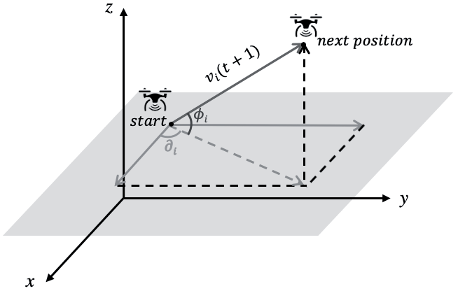
The process of using UAVs to trace air pollution sources can be divided into three phases: (I) searching for contaminant plumes, (II) tracing the source of the plume, and (III) locating the air pollution sources. We define S as the total search area, and Sk represents the area where the k-th group UAV searches for the contaminant plume. The relationship between S and Sk can be represented as S = ∑nk=1Sk. Stationi(t) = (xi(t), yi(t), zi(t))T denotes the spatial location of the i-th UAV at time t. As for the i-th UAV, the relationship between the next position and the current position can be described by Equation (3):
(3)
where xi(t), yi(t), and zi(t) (i = 1,2,3…n) are the locations of the i–th UAV in three–dimensional space at time t, and n represents the number of UAVs, respectively. In the same way, where xi(t+1), yi(t+1), zi(t+1), (i = 1,2,3…n) are the position statuses of the i–th UAV in three–dimensional inertial space at time t+1. vi(t+1) represents the velocity vector of the i-th UAV at time t+1, which is influenced by many factors, which will be discussed in more detail later in the article. φi is the elevation of vi(t+1) into the xy plane. ∂i is the azimuth at which the velocity projection of the xy plane continues to project on the x-axis, as shown in Fig. 3.
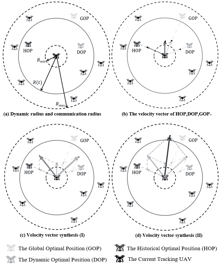
The vi(t+1) determination process is influenced by four aspects: (I) the inertial flying speed of the UAV, vi(t) ; (II) the historical optimal position (HOP) of the concentration detected during the UAV traceability process; (III) the global optimal position (GOP) of the pollutant concentration monitored by the UAV swarm; (IV) the dynamic optimal position (DOP) within the dynamic monitoring radius. It is worth noting that parameters (I)(II)(III) are the parameters in the basic PSO algorithm, but parameter (IV) has not been considered before and is, for the first time, included in the algorithm in this study. The velocity motion Equation of UAV is expressed as follows:
(4)
where w is the inertia weight, k1 and k2 are the cognitive and social learning factors in the basic PSO algorithm, and k3 is the dynamic in-domain learning factor, ri(t)~U(0,1), j = 1, 2, 3, and rj(t) represents random numbers ranging from 0 to 1. The setting of r1, r2, and r3 increases the randomness of search directions and the diversity of algorithms in the cognitive, social, and dynamic domains. w×(vix(t), viy(t), viz(t))T is the inertial flying velocity of the i-th UAV at time t and (vix(t+1), viy(t+1), viz(t+1))T is the velocity of the i-th UAV at time t+1. (xi(t), yi(t), zi(t))T is the position status of the i-th UAV at time t. (X1(t), Y1(t), Z1(t))T is the historical optimal position of the large pollutant concentration during the UAV traceability process before time t. (X2(t), Y2(t), Z2(t))T represents the global optimal position of the pollutant concentration monitored by the UAV swarm at time t. (X3(t), Y3(t), Z3(t))T represents the three-dimensional spatial position of the maximum pollutant concentration of the nearest UAV within the dynamic radius. This study marks the dynamic radius as R(t), which changes with time. The iteration of the UAV’s step length with time is shown in Fig. 4.
There are three radii in Fig. 4a): Rmax represents the maximum communication radius between a UAV and the adjacent UAV; Rmin represents the shortest distance between UAVs to avoid a collision; and R(t) represents the dynamic radius, which is influenced by the suppression psychological function that will be introduced in the later section of the article. In Fig. 4b), GOP of the UAV is the global pollutant concentration optimal position for the UAV swarm, the position of the HOP UAV is the maximum historical pollutant concentration position of The Current Tracking UAV, and DOP of the UAV represents the dynamic optimal position within the dynamic radius R(t). Moreover, Fig. 4c) and 4d) represent the process of the velocity vector synthesis, and the light-colored dot that the light-colored arrow points to is the position of The Current Tracking UAV at time t+1. With the iteration of the UAV’s step length, the concentration of air pollutants traced by the UAV gradually increases until it traces the source of the atmospheric pollutant.
Calculation of Suppression Psychological Function
As shown above, DOP of the UAV in Fig. 4 is related to the dynamic radius R(t). In this paper, we introduce the suppression psychological function to preferably study the UAV position update. The calculation of the dynamic radius R(t) depends on the suppression psychological function, which mainly considers two aspects: the state function of multiple UAVs in the group and the state function of the UAV itself.
The State Function of Multiple UAVs in the Group
When the UAV searches for pollution plumes in three-dimensional space, the influence of multiple UAVs in the group on this UAV is mainly considered from the aspects of UAV number, rank, and distance. In the MCTD control structure designed in this study (Fig. 1), there are two UAV types: (I) UAV crew and (II) dynamic UAV leaders. Thus, these different UAV types have various factors of influence (FOI) for the UAV in the group. SOI represents the influence value between two particular UAVs, and VOF is a matrix consisting of SOI that measures the degree of mutual influence between UAVs. The value of the influence matrix VOF = (SOIij)n×n is introduced as follows: the VOF between the i-th UAV and the j-th UAV, then SOIij = 0, i = n-1 represents the dynamic UAV leader, and the elements SOIij of the matrix VOF are defined by:
where n represents the number of UAVs in the k-th group, k represents the number of the UAV group. SOIijk(t) represents the influence value of the i-th UAV on the j-th UAV in the k-th group at time t. Cik(t) represents the concentration value detected by the i-th UAV crew (mg/L). Ckn–1(t) represents the concentration value detected by the dynamic UAV leader (mg/L). FOI1 and FOI2 represent the factor of influence of the UAV crew and the factor of influence of the dynamic UAV leader, respectively. Dijk is the distance between the i-th UAV and the j-th UAV in the k-th group. α is the constant factor.
Then, the total VOF value received by the i-th UAV in the k-th group at time t is as follows:
where TSOIik(t) is the total VOF value of the i-th UAV. The greater the value of influence (TSOIik), the greater the suppression psychology of the UAV created. TSOI is the total VOF value the UAV receives at a given moment, obtained by summing the SOI of the other team UAVs.
The State Function of the UAV
Besides considering the influence of other UAVs in the group, the UAV’s state function should also be evaluated. The state function of the UAV itself is mainly considered from the flight distance and remaining electricity. Because the total electric power of each UAV in the group is different, the remaining battery power (or charge level) cannot be estimated based on the flight distance. Therefore, the flight distance and the remaining battery power of the UAV should be considered separately. In order to simplify the model parameters, the relationship between the flight time of the UAV and the power is set as a simple linear relationship by the following Equation:
where a and b are constant coefficients.
The state function of the UAV is described by the following Equation:
where Gi(t) is the state function of the i-th UAV at time t. Ei(t) is the remaining battery power of the i-th UAV, Li(t) is the flight distance of the i-th UAV at time t, and β is the constant coefficient. The purpose of setting β is to prevent the denominator, also called the flight distance, from being zero when t = 0.
The Determination of Suppression Psychological Function
Considering the difference in dimension between the state function of multiple UAVs (TSOIi(t)) and the state function of the UAV (Gi(t)), the final result of suppression psychology will deviate. Therefore, the range transform method is adopted to eliminate dimension so that the result is more consistent with reality:
(9)
where
Finally, the Equation of the suppression psychological function calculation is as follows:
where Jik(t) is the suppression psychological function of the i-th UAV at time t, and w1 and w2 are weight coefficients.
The Relationship between Suppression Psychological Function and Dynamic Radius
When the “suppression” psychology of the UAV is high, it will expand the dynamic radius to obtain the plume information of the UAV in a larger field, adjust its next flight direction, and obtain high-value plume points with a higher probability. The relationship between the suppression psychological function and the dynamic radius is as follows:
where Jik(t) is the suppression psychological function of the i-th UAV, γ and ζ are constant coefficients, and γ>1 and ρ are the forgetting factors of UAV. The latter parameter is included to prevent the UAV from getting trapped in the local optimum within the search area. Rand is a random number, rand ∈[0, 1]. To better understand the behavior and performance of UVAs, random numbers are introduced in the algorithm to simulate the forgetting factor of each UAV at different times. The purpose is to examine how UVAs adjust their behavior based on their forgetting factor at different time points, such as changing search strategies or updating targets. Each UVA has a different forgetting state, and introducing random numbers can simulate the forgetting factor of each UVA at different times, thereby improving the performance and adaptability of the MCTD-DSP system.
Results and Discussion
This paper builds a three-dimensional pollution source concentration field to verify the accuracy and convergence speed of the algorithm for traceability. To validate the DSP-UAV algorithm, we run several simulations, implemented in the MATLAB simulation tool, with different configurations such as the value of k3, the number of UAVs, and the wind speeds.
Construction of the Pollution Source Field
The Gaussian pollutant diffusion model is a practical and straightforward atmospheric diffusion model that can satisfy the normal distribution of pollutant concentration in uniform and steady atmospheric turbulence. In this study, the Gaussian pollutant diffusion model was used to establish the pollutant source diffusion concentration field using the MATLAB programming language, using sulfur dioxide (SO2) as a model pollutant.
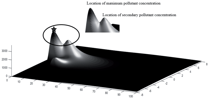
The pollution source diffusion concentration field included multiple local optimal concentration values, while SO2‘s diffusion strength concentration was 3671.6 mg/L (the position of the five-pointed star in Fig. 5).
Analysis of the DSP-UAV Algorithm
The parameters involved in the algorithm in this paper are the maximum speed of the UAV, the wind speeds, the number of UAVs, the minimum and maximum values of the dynamic radius, the four constant coefficients (w, k1, k2, k3), and the value of the psychological effect of repression. In addition, the entire contaminated area was set at 100 km×16 km to design the boundary of the simulation. These parameters were set with reference to the relevant parameters in the UAV traceability platform built by this group and in the paper, and the maximum speed of the UAV was set at 8 m/s.
The Impact of k3 and Number of UAVs on the Success Rate of Traceability
In the analysis of the DSP-UAV algorithm, the simulation parameters of UAVs and the pollution source were fixed, as presented in Table 1. The distance between UAVs must exceed the minimum communication radius to ensure collision avoidance. Dynamic leaders can also monitor the distances between UAVs and issue instructions, if necessary, to adjust their flight direction or speed to avoid collisions. It is worth noting that the value of k3 represents the importance of information in the dynamic radius and suppression of psychological function. When k3=0, the DSP-UAV algorithm is equivalent to the particle swarm optimization algorithm (PSO), which means the information within the dynamic radius is zero. Using different k3 values, 100 multi-UAV numerical simulations in the pollutant diffusion concentration map were performed in MATLAB, and the relationship between the number of UAVs and the success rate of traceability was determined (Fig. 6).
As the number of UAVs increased, the search area of the UAV group expanded, and the success rate of multi-UAV traceability to air pollution sources gradually increased (Fig. 6). When the number of multi-UAVs increased from 5 to 15, the success rate of multi-UAV traceability quickly increased, reaching the maximum of 85%. However, when the number of multi-UAVs was higher than 15, multi-UAVs were more prone to communication confusion and collision problems, resulting in a stable success rate of 85% for multi-UAV tracking, which cannot be improved further. In addition, when the number of UAVs was less than 15, the k3 value positively influenced the increased rate of the multi-UAV traceability success rate. However, when the number of multi-UAVs was greater than 15, the value of k3 did not influence the traceability success rate of multi-UAVs.
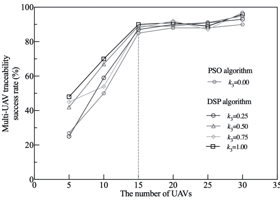
Table 1.
Simulation parameters.
| Parameters | Value |
|---|---|
| Search area | 16 km×100 km |
| Max velocity of UAV | 8 m/s |
| Number of UAVs | 5-30 |
| Longest communication radius (Rmax) | 700 m |
| Minimum communication radius (Rmin) | 10 m |
Compared to the PSO algorithm, the DSP algorithm introduces the dynamic in-domain learning factor k3. This factor allows UAVs, during the process of tracking pollution sources, to be influenced by the state functions of other UAVs in the swarm and their own individual state functions. With an increase in the psychological inhibition value of UAVs, the dynamic radius of UAVs expands, enriching environmental information within the dynamic radius. Moreover, each UAV in each group possesses a certain probability of flying towards the maximum pollutant location within the dynamic range. The DSP algorithm, to some extent, enhances the likelihood of avoiding local optima, thereby improving the success rate of retracing pollutant sources. All these aspects contribute to enhancing the convergence and success rates of UAV search operations. The comparison of the k3>0 DSP-UAV algorithm with the PSO algorithm (Fig. 6) allowed the following conclusions to be drawn: When the number of UAVs is less than 15, the PSO algorithm has a lower success rate than the k3>0 DSP-UAV algorithm; when the number of UAVs is greater than 15, the achievement rate of the PSO algorithm is similar to that of the DSP-UAV algorithm.
The Impact of Wind Speed on the Success Rate of Traceability
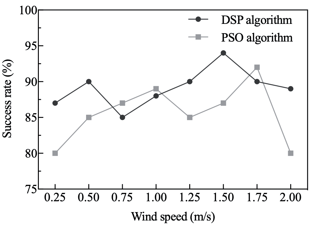
The success rates of at least one UAV locating and tracking the pollution source were further compared under different wind speeds using the PSO and DSP-UAV algorithms with 15 UAVs. The success rate of tracking was calculated by dividing the number of successful tracking attempts by the total number of attempts within a specific time frame (Fig. 7).
Fig. 7 shows that at lower wind speeds, the pollution sources did not spread widely, and the path formed by diffusion was relatively short, so the multi-UAV could not locate the pollution sources quickly along the diffusion path. Therefore, the success rate of multi-UAVs in tracking the pollution sources was low. With the increase in wind speed, the success rates of both PSO and DSP-UAV algorithms for traceability were above 80%. When the wind speed was 2 m/s, the most significant difference in traceability success rate between PSO and DSP-UAV algorithms was 9%. The wind speeds were higher at this time, and the diffusion paths of the pollution sources were easily blown around, affecting the diffusion of the pollution sources. The multi-UAVs were easily caught in the local optima and increased the multi-UAV tracking time, which would cause the multi-UAV swarm not to successfully locate the pollution sources after the iteration time was up, and the success rate of tracking decreased. When the wind speed was 0.25, 0.50, 1.25, 1.50, or 2.00 m/s, the success rate of the DSP algorithm was greater than that of the PSO algorithm; when the wind speed was 0.75, 1.00, or 1.75 m/s, the success rate of the PSO algorithm was 2%, 1%, and 2% higher than that of the DSP algorithm.
The Impact of k3 on the Convergence Speed
The relevant coefficients, k1 and k2, are the coefficients in front of the individual optimum and the population optimum of the primary particle swarm algorithm, which have already been studied in the paper and are not considered for analysis in this paper [30]. Instead, k3 is the coefficient preceding the three-dimensional spatial location of the maximum pollutant concentration within the dynamic radius for a newly proposed part. Therefore, the effect of k3 on the convergence rate was explored in this paper.
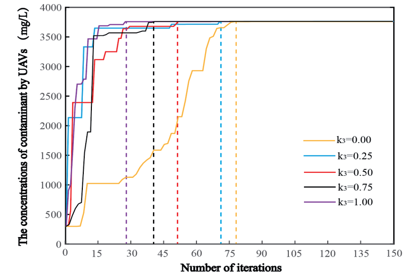
The convergence speed of the multi-UAV tracing air pollution source algorithm was estimated under the condition of using 15 UAVs, with a wind speed of 1.5 m/s and varying k3 values: k3 = 0, k3 = 0.25, k3 = 0.50, k3 = 0.75, and k3 = 1.00 (Fig. 8).
At all five values of k3, the algorithm successfully traced back to the air pollution source, and the maximum concentration of air pollution was 3671.6 mg/L. With the increase of the value of k3, the number of iterations of UAV tracing to the maximum pollution source decreased gradually. The number of iterations at k3 = 0.00, 0.25, 0.50, 0.75, and 1.00 in the DSP-UAV algorithm was 79, 71, 53, 40, and 28, respectively. It was estimated that multiple UAVs find the global optimal solution the quickest when k3 = 1.00. It should be emphasized that the greater the value of k3, the more critical the concentration information within the dynamic radius is. Under the same conditions, as the importance of information within the dynamic radius increases, the speed of tracking air pollution sources also increases. The introduction of the suppression psychological function of UAVs has important positive significance for improving the efficiency of tracing pollution sources.
While our investigation focused on the algorithm’s convergence within the range of k3 from 0 to 1, it is crucial to acknowledge potential pitfalls and drawbacks associated with continually increasing this weight. In practice, an excessively high weight for the suppression psychological function could lead to overemphasizing the concentration information within the dynamic radius, potentially causing the algorithm to become overly sensitive to local fluctuations and noise. This could result in erratic behavior and reduced accuracy in tracing airborne hazardous pollutants.
The Relationship between the Suppression Psychological Value and the Dynamic Radius
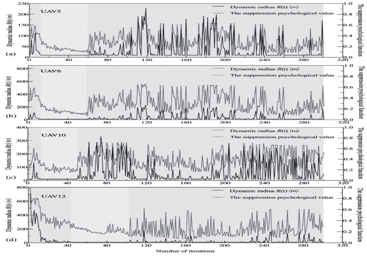
The dynamic radius of the UAV mainly depends on the value of the suppression psychological function of the UAV. The dynamic radius value is directly related to the dynamic optimal position within the dynamic radius. Under the condition that the wind speed was 1.5 m/s, k3 = 1, and the number of UAVs was 15, 4 UAVs were randomly selected from 15 UAVs to analyze the relationship between their dynamic radius and the value of suppression psychological function (Fig. 9).
In Fig. 9, the black line represents the change curve of the dynamic radius with the number of iterations. The lines of the suppression psychological value represents the change curve of the suppression psychological function with the number of iterations. The dynamic radius change trend was similar to the changing trend of the suppression psychological value (Fig. 9). However, the detailed trends of the two curves were different. This was caused by introducing the random factor (rand) in Equation (11). The purpose of setting the random factor was to randomly change the dynamic radius determined by the dynamic suppression psychological function to prevent the UAV from falling into the local optimal search area. The dynamic radius range marked by the orange background was always maintained at 10 m. This is because the minimum flight distance between UAVs was set to 10 m according to the parameters in Table 1 to prevent UAVs from colliding with each other.
Multi-UAV Traceability Process
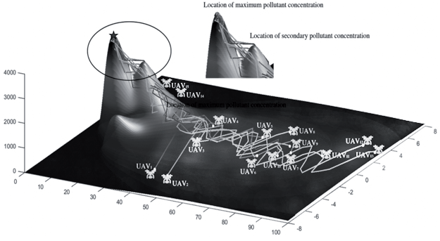
In this paper, the contribution that dynamic repression plays is represented by k3. When k3 = 0, the contribution of the dynamic repression part is zero, which is the same as the traditional PSO algorithm. When k3 = 1, the contribution of the psychological part of dynamic repression is more outstanding; i.e., as k3 increases from 0 to 1, the contribution of the dynamic repression part increases gradually. The number of UAVs is also considered in this paper. If the same time frame is used to trace the source of pollution, the lower the number of UAVs, i.e., the lower the cost required. Section “The Impact of k3 and Number of UAVs on the Success Rate of Traceability” examines the impact of the number of UAVs on the success rate of traceability, which shows that a number of UAVs around 15 has excellent results; when there are fewer than 15, the success rate of traceability gradually decreases. Under these conditions, the simulation of the traceability path of multiple UAVs was conducted (Fig. 10).
Fig. 10 shows the multi-UAV traceability control roadmap at k3 = 1.0. In the beginning, many UAVs are scattered in the search area (white dots). Then, groups of UAVs within a dynamic radius interact with each other to share information about monitored pollutant concentrations, often making the groups of UAVs fly in the direction of high concentrations. After a period of time, some UAVs search for and trace the plume of pollutants to the source of air pollution. In addition, the DSP-UAV algorithm can successfully trace the source of air pollution. The location of the red pentagram is the maximum spatial location for multi-UAV to trace the pollution source concentration point. Some UAVs pass through the second pollution concentration peak and then fly to the peak of maximum pollutant concentration. This shows that the DSP-UAV algorithm has the advantage of avoiding the fall into local optima.
According to the above numerical simulation and analysis, this DSP-UAV algorithm has a faster convergence speed than the traditional particle swarm optimization algorithm. It can also avoid falling into the local optima. The DSP-UAV algorithm has good prospects for using multiple UAVs to trace the source of atmospheric pollution.
Discussion
The proposed MCTD control structure and DSP-UAV algorithm have achieved significant results in collaboratively tracking pollution sources, using sulfur dioxide (SO2) as the model pollutant. The pollutant dispersion intensity concentration is 3671.6 mg/L, covering an area of 100 km×16 km. The drones’ maximum speed is 8 m/s, and the minimum flying distance between them is 10 meters.
The DSP algorithm introduces a dynamic intra-domain learning factor, k3, ranging from 0 to 1, to avoid excessive suppression of the psychophysical function weights, which can lead to unstable behavior and reduced accuracy when tracking harmful pollutants in the air. This factor allows the drones to be influenced by the state functions of other drones in the group and their own state functions while tracking the pollution source. Increasing the value of k3 expands the dynamic radius of the drones, allowing them to gather more environmental information and improve the tracking success rate. When k3=1.00, multiple drones can quickly find the global optimal solution. The positive impact of k3 on the tracking success rate is more significant when the number of drones is less than 15. However, when the number of drones exceeds 15, the impact of k3 on the tracking success rate becomes less significant. This indicates that the value of k3 needs to be adjusted based on the number of drones and the actual scenario to achieve the best tracking effect.
Under low wind speed conditions, the diffusion range of the pollution source is limited, making it difficult for multiple drones to locate the source quickly and resulting in a lower tracking success rate. As wind speed increases, the PSO and DSP-UAV algorithms show improved tracking success rates. However, excessive wind speed can cause chaotic dispersion paths for the pollution source, increase the risk of drones getting stuck in local optima, and decrease the tracking success rate. This indicates the need to consider the influence of wind speed on the tracking process and select appropriate wind speed conditions for tracking in practical applications.
The higher the number of drones, the larger the search range and the higher the tracking success rate, but cost factors also need to be considered. Experimental results show that 15 drones achieve the highest tracking success rate, with relatively low costs. This provides a reference for selecting the number of drones in practical applications.
Compared to the traditional PSO algorithm, this study introduces the maximum pollution three-dimensional spatial position within the dynamic radius range of the drones in the MCTD control structure for multi-drone cluster tracking. This method aligns well with the actual application scenarios of drones and improves algorithm performance. The DSP-UAV algorithm exhibits a higher success rate of tracking under wind speeds of 1.5 m/s, k3=1, and 15 drones, effectively avoiding getting stuck in local optima during the tracking process, thereby improving tracking efficiency.
The MCTD control structure and DSP-UAV algorithm provide an effective method for the collaborative tracking of pollution sources by multiple drones and have practical application value. This study provides technical support for air pollution control and management and indicates directions for future research. In addition, digital watermarking technology is utilized to embed representative identification information (i.e., digital watermarking) into a digital carrier, which can transmit secret messages and judge whether digital content has been tampered with [36]. With reference to the principle of digital watermarking technology, the data transmission function of the MCTD control structure is modified, and the data information coming from the UAV is labeled using digital watermarking technology, which may improve the data processing efficiency of the ground control station and enhance the data reliability at the same time.
Conclusions
In this study, we designed an MCTD control structure for UAVs, which solves the issue of the limited flight time and communication range of the UAVs in a large area of source traceability. Specifically, this study proposed a DSP-UAV algorithm introducing social impact theory to UAV manipulation and control. It was shown that the UAV obtains the local optimal value within the dynamic radius and avoids wasting resources caused by frequent transitions of UAVs when relying on the global optimal search. As the number of UAVs increases and is less than or equal to 15, the tracking success rate is significantly improved, and the DSP-UAV algorithm with k3>0 is superior to the traditional PSO algorithm. The significant difference between the proposed DSP-UAV algorithm and the traditional UAV search algorithm is that it creatively presents detecting the optimal pollutant concentration within the dynamic radius, which can effectively avoid falling into the local optima with good convergence speed. Future research directions should include the communication processing mechanism of multiple UAVs in emergencies, formation control of multiple drones, design of obstacle avoidance strategies, and consideration of additional meteorological conditions and pollutant diffusion rates, which will ensure that multiple UAVs can effectively collaborate and enhance their coordination and tracking efficiency in complex environments. Meanwhile, it is essential to ensure the safety and reliability of drones during the tracking process and further validate the effectiveness and robustness of the algorithms. Validation of the proposed MCTD control structure and DSP algorithm in real-world scenarios will be essential, incorporating a more comprehensive range of meteorological conditions and pollutant dispersion rates into our experimental framework. Continuous DSP algorithm refinement is warranted to dynamically adapt to evolving environmental factors, ensuring its robustness and efficacy across diverse meteorological conditions and pollutant dispersion rates.
In the future, we will continue to design more reliable and robust inter-UAV communication mechanisms to ensure that UAV swarms can maintain effective communication in emergency situations and respond quickly to emergencies; study more flexible and adaptive UAV formation flight strategies to enable UAV swarms to collaborate effectively in different environments and mission requirements; develop more accurate and safe UAV obstacle avoidance algorithms to ensure that UAV swarms in the process of performing their missions can avoid obstacles and ensure the safety of personnel and equipment; consider the effects of more meteorological conditions and pollutant dispersion rates, such as wind direction, wind speed, temperature, humidity, etc., and build corresponding models to improve the accuracy and adaptability of the algorithms; and apply artificial intelligence and machine learning technologies to the control and search strategies of UAV swarms, e.g., using deep learning algorithms to learn the characteristics of cloud clusters and predict the trend of their dispersion. It is of utmost importance to validate the proposed MCTD control structure and DSP algorithm in real scenarios and conduct more extensive experiments, e.g., testing under different meteorological conditions and pollutant diffusion rates, to ensure the effectiveness and robustness of the algorithm.