

Introduction
Evapotranspiration (ET) is a crucial component of ecosystem water, energy, and biogeochemical cycles. They play a key role in effectively allocating and managing regional water resources [1-3]. Owing to the impacts of climate change and human activities, water scarcity has become a significant constraint on the sustainable development of arid and semi-arid areas [4]. The accurate estimation of evapotranspiration provides a theoretical and scientific foundation for ecological restoration and management of water resources in these regions [5, 6].
Global climate change has caused significant modifications to eco-hydrological processes, with particular emphasis on evapotranspiration. This has garnered substantial attention and noteworthy achievements from scholars worldwide [7]. Xue Jingyuan et al. conducted studies comparing daily crop ET in California’s Central Valley using the METRIC, SSEB, and SEBAL models [8]. Lian Jinjiao et al. evaluated the performance of the METRIC, SEBS, and TS-VI triangular models in the middle reaches of the Heihe River Basin [9]. Numerous comparisons between single-source and dual-source models have been conducted in irrigated agricultural regions with semi-humid climates [10, 11]. These studies have involved the comparison and validation of model results with observations from eddy covariance systems and the performance of sensitivity analyses on model inputs [12, 13]. The complexity of surface characteristics and climate in arid regions has posed challenges in parameter estimation for these models, further complicating ET studies [14, 15].
The Horqin Sandy Land, one of China’s largest sandy areas, represents a typical arid and semi-arid region. The quantification of ET in this region has presented a formidable challenge owing to intricate hydrological processes and underlying surface characteristics [16]. With the rapid development of remote sensing technology, innovative methods that combine physical principles with remote data have provided novel approaches for obtaining regional-scale energy flux. The surface energy balance principle that has been widely employed for ET estimation can calculate the latent heat flux (LE) as the residual term after determining the sensible heat flux (H) through surface parameters [17-19]. Energy balance models can be into divided two categories: single- and dual-source models [20-22]. Remote sensing-based single-source energy balance models, such as the Surface Energy Balance Algorithm for Land (SEBAL) and Mapping Evapotranspiration at High Resolution with Internalized Calibration (METRIC), primarily rely on the VI-ST relationship to model energy flux, treating the surface as a whole without distinguishing soil from canopy. By constraining the temperature endmembers, the coldest endmember denotes conditions near potential ET, whereas the hottest endmember represents units near the minimum latent heat flux [23-25]. In contrast, dual-source models rely on surface temperatures of soil and canopy, which cannot be directly accessible from satellite images. Researchers at home and abroad have extensively explored methods to decompose surface temperatures into vegetation and canopy temperatures [26-28]. The classical Two-Source Energy Balance (TSEB) model employs the Priestley-Taylor (P-T) parameterization method to iteratively calculate soil and canopy temperatures. Energy fluxes among the soil surface, vegetation canopy, and atmosphere can be simulated using parameters and constants derived from remote sensing, allowing the estimation of transpiration and evaporation from both surfaces [29-31]. However, comprehensive comparisons between single-source and dual-source models in the intricate environments of arid and semi-arid regions remain limited. A deeper understanding of the energy flux simulation differences stemming from the distinct physical mechanisms of these models is needed [32, 33].
This study employed two surface energy balance-based ET models to simulate energy flux during the 2018-2022 growing season in the study area. The TSEB and METRIC models were validated using eddy covariance systems and large-aperture scintillometers. The objectives of this study included establishing ET models suitable for arid and semi-arid regions, elucidating spatiotemporal ET patterns, exploring the impact of model input data on regional ET, and clarifying the driving mechanisms behind regional evapotranspiration.
Materials and Methods
Study Area
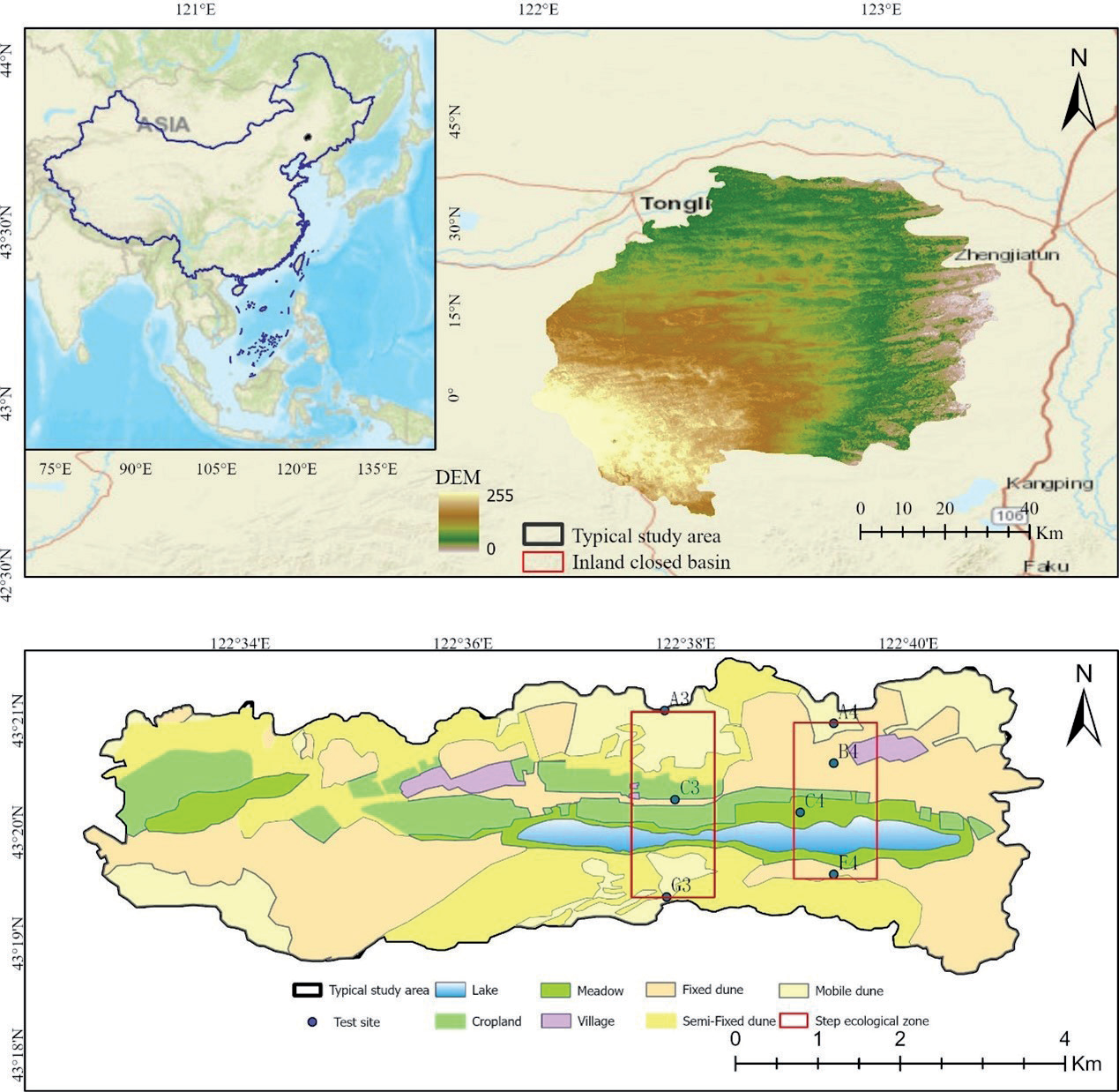
The study area is located in an inland closed basin at the southeastern edge of the Horqin Sandy Land (42°40′-43°42′ N, 122°00′-123°20′ E), which falls under the administrative jurisdiction of Keerqin Zuoqi, Tongliao City, Inner Mongolia Autonomous Region. Covering approximately 8,000 km2, the typical study area encompasses 55 km2 (Fig. 1). Topographically, the region follows a west-high, east-low, north-high, and central-low pattern. It features a landscape characterized by alternating sand dunes and grasslands, marked by a patchy distribution of vegetation, displaying significant spatial heterogeneity. Shrub and semi-shrub species such as Caragana microphylla and Artemisia halodendron Turcz et al. Bess primarily covers the sand dunes, while the meadows consist mainly of grasses from the Stipa genus and various Asteraceae species. The study area experiences a temperate continental semi-arid climate, with an annual precipitation range of 300-400 mm, 70% of which occurs between July and September. This study focused on the A4 dune ecosystem and C4 cropland ecosystem within a typical area, along with two dune-cropland ecotones, which were point-scale and regional-scale model validation sites (Fig. 1).
Data Sources
Remote Sensing Data
For the METRIC and TSEB models in this study, the input data required high-resolution, cloud-free satellite imagery and conventional meteorological information. Multispectral satellite images with a spatial resolution of 30 m were obtained from the United States Geological Survey (USGS) (https://www.usgs.gov/). These images provided spectral data in 11 bands with a temporal resolution of 16 d. Specifically, for model inputs, the Band 4 (Red) and Band 5 (Near-Infrared, NIR) of Landsat 8 Level-2 products were selected. These bands were utilized to calculate the normalized difference vegetation index (NDVI), vegetation cover fraction (FVC), and leaf area index (LAI). Additionally, Band 10 (10.60-11.19 μm) was selected for land surface temperature (LST) inversion.
Digital Elevation Model (DEM) data with a 30-meter resolution were obtained from the Shuttle Radar Topography Mission (SRTM) via the USGS website. Table 1 presents the selection of 15 Landsat 8 images (Path/Row 120/30) without cloud cover between September 2018 and October 2022. These images consisted of 3 from 2018, 2 from 2019, 2 from 2020, 3 from 2021, and 5 from 2022, with acquisition times specified in Greenwich Mean Time (GMT). The crop planting cycle in the research area is specified in the early stages of vegetation growth in May and June. July and August are the middle periods of vegetation growth, and September and October are the late periods of vegetation growth.
Meteorological Data
The meteorological data utilized in this study primarily originated from the NASA Global Land Data Assimilation System (GLDAS), accessible at https:// disc.gsfc.nasa.gov/. GLDAS employed multiple offline land surface models that integrated extensive ground observation data at a global scale with high resolution. Specifically, the GLDAS_NOAH05_3H_2.1 data were selected, with a temporal resolution of 3 h and a spatial resolution of 0.25° × 0.25°. The selected meteorological variables included air temperature, pressure, wind speed, and shortwave radiation.
Table 1.
Selected Landsat8 images from 2018 to 2022.
Eddy Covariance Data
In the specified region, two sets of long-term eddy covariance systems were installed in the dune ecosystem (A4) and cropland ecosystem (C4). These systems were equipped with state-of-the-art components, including three-dimensional ultrasonic anemometers (CAST-3, Campbell Scientific, USA) and thermal infrared gas analyzers (LI-7500, Li-Cor Inc., Nebraska, USA). Their primary function was to measure the water-heat-carbon fluxes in both sand dune and grassland ecosystems. Furthermore, these systems incorporated additional instruments, such as four-component net radiometers and soil heat flux plates, to accurately measure net radiation and soil heat flux.
Large-Aperture Scintillometer Data
Within the designated area, two large-aperture scintillometers (LAS) were deployed to monitor sensible heat flux profiles along three and four lines (Fig. 1). These profiles encompassed various ecosystems, such as mobile sand dunes, semi-fixed sand dunes, fixed sand dunes, grassland farmland, and grassland wetlands. Together, these ecosystems constituted a comprehensive sand dune-grassland ecotone aligned in a north-south direction (Fig. 1).
Data Processing
Remote Sensing Data
Use the Python programming language combined with the Kriging interpolation method to perform batch processing of GLDAS meteorological raster data. This method can standardize the spatial coordinate system of remote sensing and meteorological raster data to 30 m, ensuring that the image size and coordinate system are consistent.
The Google Earth Engine platform (https:// earthengine.google.com/) was applied to perform cloud removal on Landsat 8 data. Subsequently, remote sensing parameters such as NDVI, FVC, and LAI essential for the models were calculated. The formula is as follows:
Vegetation cover was determined through a pixel dichotomy method, where NDVIsoil values were selected to approximate the accumulated 5% of NDVI, and NDVIveg values were chosen to approximate the accumulated 95% of NDVI. Confidence intervals could be adjusted to account for differing vegetation conditions across various regions.
Flux Data
The eddy covariance flux data underwent comprehensive correction processes utilizing the EddyPro flux data processing software developed by Li-COR. These corrections included the elimination of anomalies and outliers, tilt correction, Webb Pearman Leuning correction, and a sequence of other necessary adjustments, resulting in flux data on a half-hourly scale. Subsequently, further quality control measures, such as turbulence characteristic assessments and stationarity checks, were implemented. Missing flux data were interpolated to ensure the accuracy and continuity of the dataset. Additionally, the energy closure ratio of eddy covariance systems was calculated using the energy balance ratio [16].
Initially, Large-Aperture Scintillometer (LAS) data were collected at 1-minute intervals. These raw data underwent several processing steps, including data exclusion, filtering, interpolation, correction, and averaging, to yield sensible heat flux data on a 30-minute scale.
Model Evaluation
In order to evaluate the performance of the two models, the results were compared using error components such as coefficient of determination R², root mean square error RMSE, standard deviation SD, and mean absolute percentage deviation MAPE.
In the formula, O and P represent the actual value and simulated value, respectively, and n is the number of data samples considered.
Models
Combined with the TSEB and the METRIC models, Landsat series satellite remote sensing data were utilized for estimating evapotranspiration in the study area. Both the TSEB and METRIC models were based on the surface energy balance principle to estimate the regional ET.
In these models, LE represents latent heat flux, Rn is the net radiation flux, G is soil heat flux, and H is sensible heat flux (W/m²). In Equation (8), it was assumed that other energy terms, such as thermal advection, canopy heat storage, and photosynthetic energy, could be considered negligible. The determination of the LE was not a direct measurement achievable through remote sensing; instead, it can often be computed as the residual in the energy balance equation.
TSEB Model
The TSEB-PT model primarily relied on remotely sensed land surface temperature data acquired through vertical observations of the Landsat 8 satellite. This temperature data was applied as the model input and utilized the Priestley-Taylor (PT) formulation to iteratively estimate soil and canopy component temperatures. In the TSEB model, the directional radiative temperature (Trad) was predominantly affected by soil temperature, vegetation temperature, and vegetation cover fraction, and its formulation is expressed as follows:
where Tc and Ts represent the canopy temperature (K) and soil temperature (K), respectively, and Trad is the radiative temperature. By combining canopy and soil temperature with data on other energy fluxes, net radiation for the vegetation canopy (Rnc) and net radiation for the soil surface (Rns) can be calculated separately.
In Equations (10) and (11), subscripts “s” and “c” represent soil and vegetation components, respectively; τ, ε, and α denote radiation transmissivity, emissivity, and reflectivity, respectively; S↓ and L↓ represent incoming shortwave and longwave radiation, respectively; subscripts “longware” and “solar” represent longwave and shortwave, respectively. G0 is the soil heat flux, and G/Rn is an empirical constant. The actual value of G/Rn varies for different vegetation types. The soil heat flux G0 is calculated as follows:
In Equation (12), a, b, and c represent the defined maximum ratio (a = 0.35), sine curve shape (b = 8000s), and phase shift of the sine curve (c = 3600s) [16], respectively.
The sensible heat flux H can be calculated using the following formula:
In Equations (13) to (15), ρ is air density; Cp is the volumetric heat capacity of air; TAc is the air temperature within the vegetation air layer; RX (sm⁻¹) is the total boundary layer resistance of the canopy; RS (sm⁻¹) is the total boundary layer resistance at the soil surface; and RA (sm⁻¹) is the total boundary layer resistance in the air. The sensible heat flux from the soil (canopy) was calculated based on the gradient between the soil (canopy) and air temperatures within the vegetation air layer. RX, RS, and RA were computed using the method proposed by Norman and Kustas [34].
In the TSEB-PT model, Ts and Tc are a priori unknown, and it is initially necessary to calculate the potential rates using the green vegetation fraction (fg) and the Priestley-Taylor formula:
where αPT represents the Priestley-Taylor coefficient, initially set to 1.26, fg is the proportion of green vegetation, Δ is the slope of saturation vapor pressure with respect to temperature, and λ is the latent heat constant. Subsequently, the canopy temperature (Tc) was calculated by inverting the turbulent heat transfer equation between the surface and the reference height above the surface. The soil temperature was computed using Equation (9), and the soil sensible and latent heat fluxes were then determined.
During the computation, if the soil latent heat flux is non-negative, it is solved; otherwise, canopy transpiration decreases with a reduction in αPT, effectively increasing Tc and lowering Ts until a feasible solution is found (no negative condensation values for λE on either soil or canopy) [35]. Finally, latent heat fluxes for the soil and vegetation surfaces are calculated based on the energy balance equations for the vegetation and soil surfaces.
Upon acquiring the instantaneous latent heat flux, a crucial step was to scale the time required to compute the daily ET. This process assumed that the ratio of the estimated instantaneous latent heat flux to RS at transit time remained constant throughout the day. Solar radiation data were utilized in conjunction with this assumption to generate daily ET data.
where ETd represents the estimated daily evapotranspiration (mm/day); LE is the latent heat flux at the satellite transit time (W/m²); Rd is the daily downward shortwave radiation on a daily time scale (MJ m⁻²day⁻¹); λ is the latent heat of vaporization (MJ kg⁻¹); RS is the downward shortwave radiation at the satellite transit time (W/m²); and ρω is the density of water (kg m⁻³).
METRIC Model
The METRIC model, an improvement of the SEBAL model by Allen et al. (2007), utilizes the ESA algorithm to identify endmember pixels in satellite images. This enables the determination of energy balance conditions for both cold and hot pixels, facilitating the ET calculation. The model employs remote sensing data from various spectral bands in satellite images to compute the effective energy terms, which are then related to ET via the residual of the surface energy balance (Equation 4). To ensure a fair assessment of the performance of the model in ET estimation, both models are supplied with identical sets of meteorological and remote sensing data.
In the METRIC model, the soil heat flux (G) was estimated by applying the formula established by Bastiaanssen and Wright. This calculation considered root reflectance, land surface temperature (LST), and the normalized difference vegetation index (NDVI) [36, 37]:
In Equation (20), T represents the land surface temperature (K), and α is the surface reflectance. Tasumi replaced the original formula for calculating soil heat flux in METRIC with that developed by Wright [38]. The formula used is as follows:
METRIC and SEBAL diverge in their approaches to solving the sensible heat flux, especially in their methods of calibrating the solution for individual satellite images. The estimation of the sensible heat flux (H) primarily relies on aerodynamic functions:
In Equation (23), ρair is the air density (kg/m³); Cp is the specific heat of air at constant pressure (Jkg⁻¹K⁻¹); γah is the aerodynamic resistance between two near-surface heights (sm⁻¹); Z1 and Z2 are typically set to 0.1 and 0.2 m, serving as parameters for calculating aerodynamic roughness for a specific pixel; and dT (K) represents the near-surface temperature difference between Z1 and Z2.
The primary emphasis of this model was on utilizing the ESA algorithm to enhance the selection of endmember pixels within the METRIC model [39]. This improvement was achieved through an automated procedure proposed for the selection of both thermal and cold pixels [40].
Results and Discussion
Validation of Site-Scale Model Accuracy
In this study, the accuracies of the METRIC and TSEB models were assessed in simulating net radiation, soil heat flux, latent heat flux, and sensible heat flux using data from eddy covariance systems. The results are presented in Table 2. For the METRIC model, RMSE values for net radiation simulations in the meadow ecosystem and dune ecosystem were 91.26 W/m² and 94.89 W/m², SD values were 103.04 W/m² and 102.32 W/m², MAPE values were 7% for both, and R² values were 0.937 and 0.913, respectively. For soil heat flux simulations, RMSE values were 23.52 W/m² and 36.65 W/m², SD values were 32.95 W/m² and 50.65 W/m², MAPE values were 17% and 33%, and R² values were 0.586 and 0.67, respectively. In the case of sensible heat flux simulations, RMSE values were 51.32 W/m² and 57.42 W/m², SD values were 79.36 W/m² and 86.41 W/m², MAPE values were 51% and 26%, and R² values were 0.638 and 0.639, respectively. Finally, for the latent heat flux simulations, the RMSE values were 27.79 W/m² and 30.86 W/m², SD values were 81.31 W/m² and 24.6 W/m², MAPE values were 12% and 39%, and R² values were 0.893 and 0.395, respectively.
The TSEB model yielded the following results for net radiation simulations in the meadow ecosystem and dune ecosystem: RMSE of 96.49 W/m² and 89.32 W/m², SD of 102.09 W/m² and 101.67 W/m², MAPE of 7% and 6%, and R² values of 0.931 and 0.932, respectively. For soil heat flux simulations, RMSE values were 22.85 W/m² and 40.52 W/m², SD values were 40.89 W/m² and 40.09 W/m², MAPE values were 18% and 33%, and R² values were 0.761 and 0.559, respectively. In terms of sensible heat flux simulations, RMSE values were 31.42 W/m² and 41.10 W/m², SD values were 44.78 W/m² and 61.02 W/m², MAPE values were 69% and 20%, and R² values were 0.603 and 0.761, respectively. Finally, for the latent heat flux simulations, RMSE values were 45.74 W/m² and 15.99 W/m², SD values were 74.49 W/m² and 40.79 W/m², MAPE values were 20% and 26%, and R² values were 0.809 and 0.865, respectively.
The core of the energy balance equation revolved around the calculation of LE, with the accuracy of determining Rn, G, and H directly affecting the results of the models. The accurate simulation of net radiation, which was a vital energy balance component, was of great significance. In both models, the RMSE range for Rn at the ecosystem level spanned from 89.32 W/m² to 96.49 W/m², indicating relatively larger errors than other energy components. This may be attributed to the inherent complexity of underlying surfaces in arid and semi-arid regions, affecting surface radiation characteristics, emissivity, and reflectance, which affected the proportion of crop photosynthetically active radiation and the surface energy balance. Notably, Horton et al. revealed that crop residues could alter surface evaporation and soil moisture, thereby affecting shortwave reflectance and longwave emissivity and consequently influencing net radiation [41]. G constitutes a relatively minor component of the energy balance, representing the available energy allocated to sensible and latent heat fluxes. Accurate G estimation can often be challenging because of variations in soil moisture and vegetation. Singh et al. observed low R² values for estimated soil heat flux at three different locations in the central United States (0.03, 0.36, and 0.33) [42]. Irmak et al. utilized different remote sensing models to estimate soil heat flux in Nebraska, yielding variations ranging from 36.3 W/m² to 62.6 W/m² due to differences in soil properties, sensor depth, and sensor spacing [43]. Notably, Bastiaanssen and Wright improved the soil heat flux formula in the METRIC model by introducing the leaf area index [36, 37]. According to equation (12), the parameter a in the TSEB model is set to 0.4, which significantly improves the accuracy of soil heat flux simulations in the TSEB and METRIC models. The R² values for soil heat flux estimates ranged from 0.559 to 0.761, with RMSE values ranging from 23.52 W/m² to 50.65 W/m².
Accurate estimation of H is of paramount importance in energy balance models. Notably, the METRIC model tended to overestimate the H across both ecosystem scales, resulting in RMSE values of 51.32 W/m²–57.42 W/m². Conversely, the TSEB model provided a more precise estimation of H, with RMSE values spanning from 31.42 W/m² to 41.1 W/m². These differences in the results can be attributed to the different formulas employed by each model. The accuracy of the METRIC model depends significantly on the proper selection of hot and cold pixels during the calibration process for a given image. METRIC utilizes an internal calibration procedure to estimate the near-surface temperature gradient (dT) as an indicator of the radiometric surface temperature (TS), thereby facilitating the estimation of the H. The METRIC model did not consider parameters such as stomatal resistance and employed a single surface temperature. Under high surface temperatures, the H value for dry bare soil reached its maximum, whereas, in low-temperature scenarios, the H value for moist vegetation approached zero. However, when extreme points (dry and wet) were absent, the METRIC model faced challenges in accurately simulating the H owing to its sensitivity to the temperature difference between these two extremes [25, 26]. The findings are presented in Fig. 2 and Fig. 3, the TSEB model exhibited an overestimation of the sensible heat flux in the grassland ecosystem and an underestimation in the dune ecosystem. This discrepancy was attributed to the sparse vegetation in the dune ecosystem, where water stress on vegetation led to limitations in the ability of the P-T coefficient αPT to accurately capture the extent of water restriction on vegetation transpiration [44]. This factor may significantly contribute to the underestimation of H in dune ecosystems. The TSEB model emerged as a more reliable estimator of sensible heat flux than the METRIC model at both ecosystem scales.
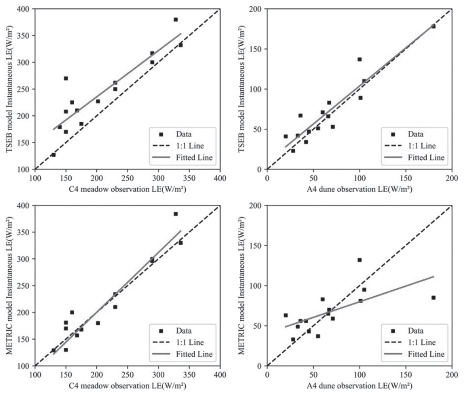
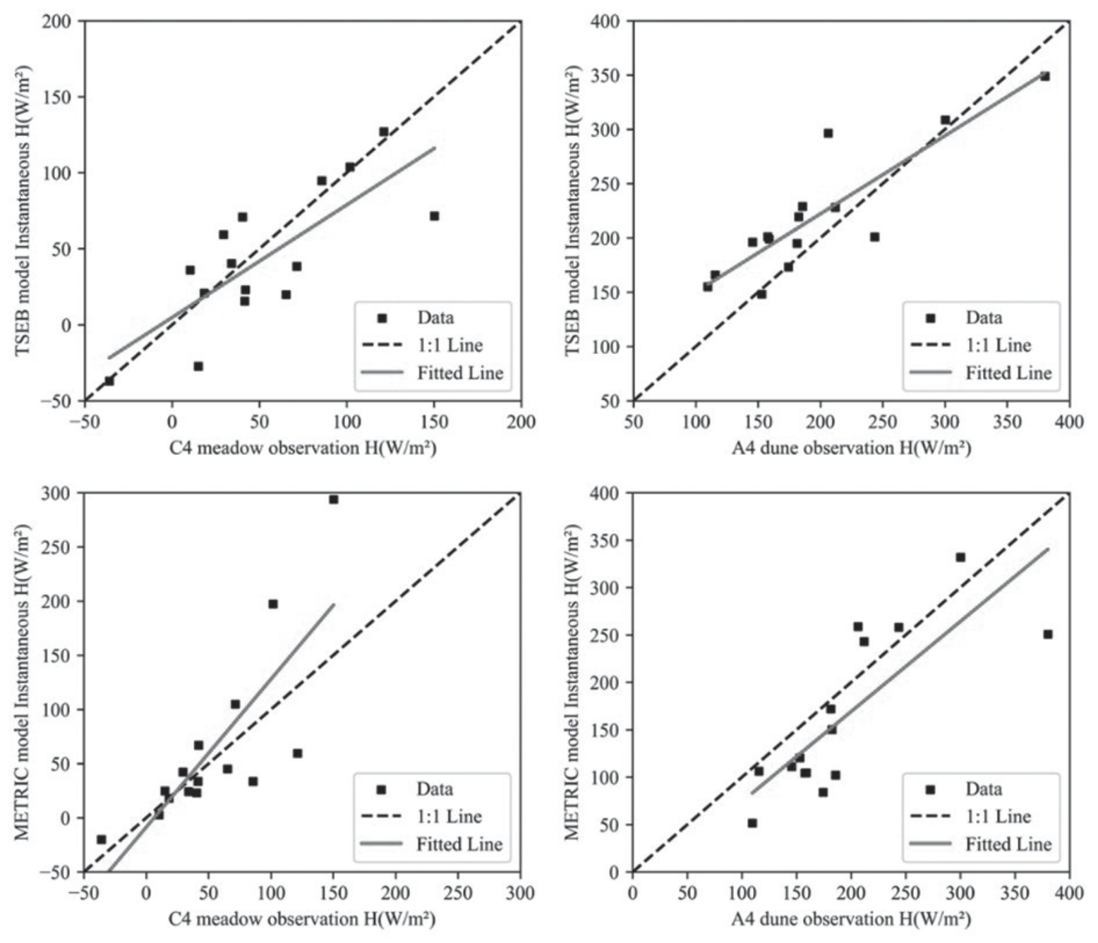
Table 2.
Vorticity data validation of the METRIC and TSEB models.
At the ecosystem scale, the METRIC model tended to overestimate the H, whereas the TSEB model exhibited superior performance in simulating the H. Furthermore, the TSEB model displayed higher accuracy in simulating the latent heat flux (LE) in sparsely vegetated regions than the METRIC model. Conversely, the METRIC model outperformed the TSEB model in simulating LE within a meadow ecosystem. These findings were consistent with those of Xu Yanhao and Wim J. Timmermans, suggesting the conclusion that the TSEB model can provide more dependable LE estimates under conditions characterized by dry soil surfaces and limited vegetation cover [45, 46].
Verification of Regional-Scale Model Accuracy
In this study, regional-scale validation was conducted by comparing Large-Aperture Scintillometer (LAS) observation data with model-generated results within the 3-line and 4-line sand-dune-meadow gradient ecological zones. The findings are presented in Fig. 4 and Table 3. Specifically, for the METRIC model, the RMSE of simulated H on the 3-line and 4-line zones were 67.97 W/m² and 49.47 W/m², SD values were 84.69 W/m² and 73.55 W/m², MAPE values were 33% and 32%, R2 values were 0.51 and 0.652, respectively. In contrast, the TSEB model exhibited RMSE values of 43.28 W/m² and 22.83 W/m² for simulated sensible heat flux on the 3-line and 4-line zones, SD values of 42.43 W/m² and 36.05 W/m², MAPE values of 14% and 17%, and R2 values of 0.656 and 0.681, respectively.
Comparative studies involving Large-Aperture Scintillometer data and remote sensing ET models were notably limited, they typically focused on comparing Large-Aperture Scintillometer data with measurements from eddy covariance sites [47, 48]. The TSEB model exhibited a regional H simulation with RMSE values ranging from 22.83 W/m² to 44.83 W/m², while the METRIC model simulated regional H with RMSE values spanning from 49.47 W/m² to 67.97 W/m². Both models demonstrated commendable performance in simulating H at both regional and ecosystem scales. These findings were consistent with those of Semeh et al., who utilized the SPARSE model to calculate instantaneous H and LE at the time of satellite overpass, suggesting a strong correlation between LAS-measured H and satellite-estimated instantaneous H [49]. In summary, both the TSEB and METRIC models tended to underestimate the regional H, a phenomenon potentially attributed to disparities between simulated regional scales and the actual distribution of source areas [50, 51].
Spatial and Temporal Distribution of ET
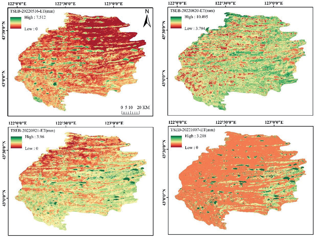
Fig. 5 illustrates the spatial distribution of ET as simulated by the TSEB model within the study area. Using the TSEB model, we derived the 30-meter spatial distribution of ET for the year 2022. On specific dates, namely May 16, August 20, September 21, and October 7, 2022, the simulated daily ET exhibited the following ranges: 0-7.512 mm, 3.794-10.495 mm, 0-3.96 mm, and 0-3.128 mm, respectively. Notably, ET presented a distinct seasonal pattern characterized by rapid growth during the early period, reaching its zenith in August and subsequently decreasing in September and October. In May, the spatial distribution was uniform, with the highest ET values observed over the lake. In August, a pronounced east-high and west-low pattern emerged, whereas, in September, a northwest-low and southeast-high pattern became evident. Notably, in the southeast, where crops such as corn and rice were cultivated, there was a substantial reduction in ET during early October as these crops approached maturity.
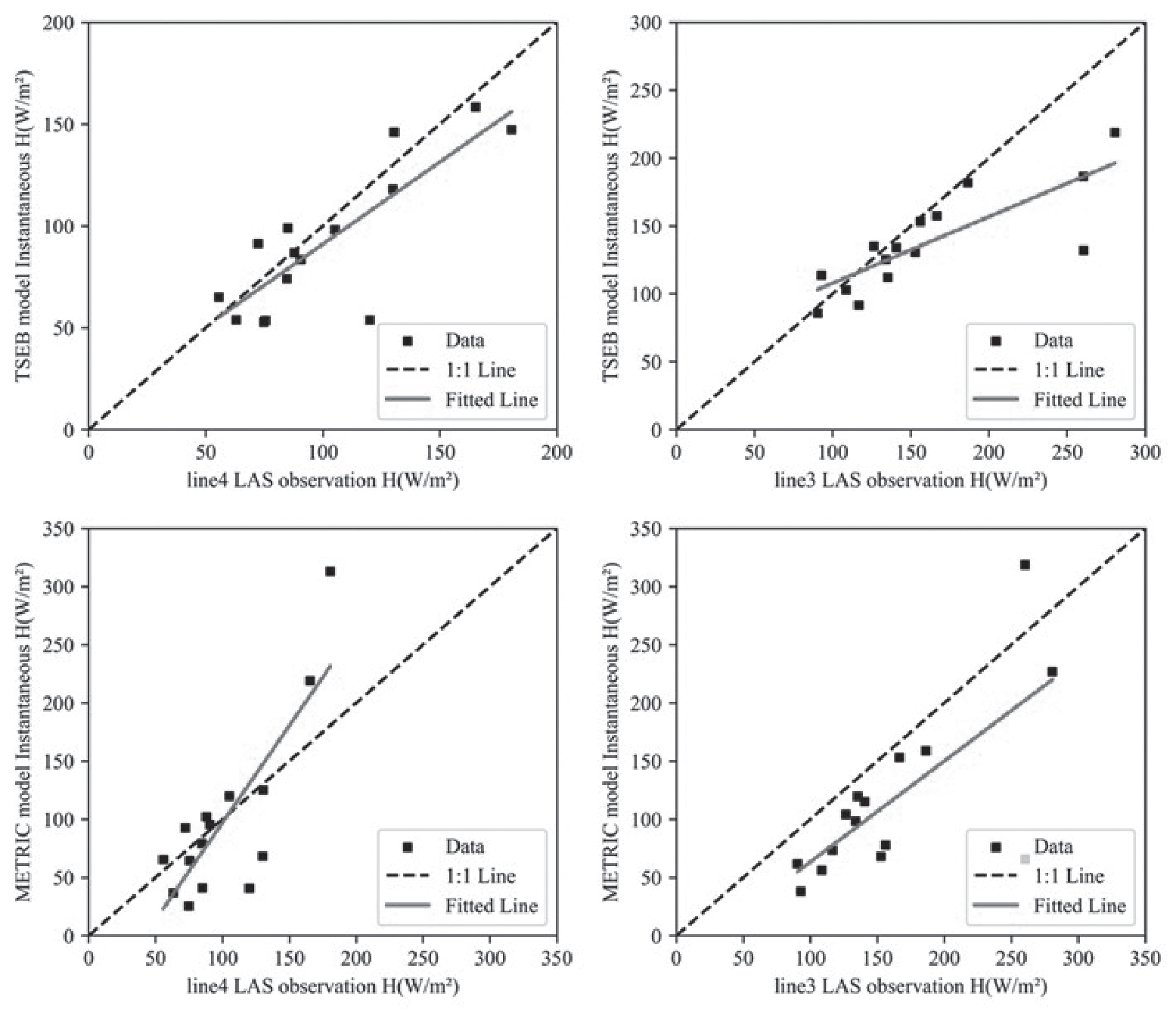
Table 3.
LAS data validation of METRIC and TSEB models.
Distinct variations in ET spatial patterns were discernible across different land cover types. The order of ET distribution, from highest to lowest, was lake> grassland>wetland>rice>corn>sand dune>urban area, as determined by the TSEB model. This result was consistent with the findings of Jamal Elfarkh et al. [52].
Driving Factors of ET
A comprehensive analysis was conducted by comparing three key model input factors in relation to ET: LAI, LST, and temperature differential between land surface and air (ΔT). The results revealed a pattern in ET behavior, with an initial rise followed by a decline as the LAI changed throughout the growing season (Fig. 6). The ET reached its zenith in August. The LST exhibited a peak in May and a gradual decrease from August to October. Notably, during the later stages of vegetation growth, ET displayed sensitivity to variations in ΔT in response to fluctuations in this parameter.
To gain a deeper understanding of the impacts of the three input factors on regional ET, we computed the spatial correlations of these variables with ET for cloud cover images below 10% from 2018 to 2022 (Fig. 7). These findings highlighted the significant impact of the LAI and the ΔT on ET within the study area. The correlation between ΔT and ET mirrored that of the Digital Elevation Model (DEM), where ΔT and ET exhibited a negative correlation ranging from 0 to -0.93, whereas in low DEM regions, ΔT and ET displayed a positive correlation ranging from 0 to 0.77. Additionally, the LAI consistently demonstrated a strong positive correlation throughout the entire region, ranging from 0 to 0.9.
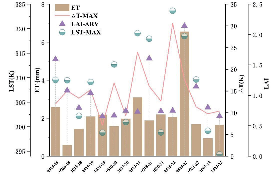
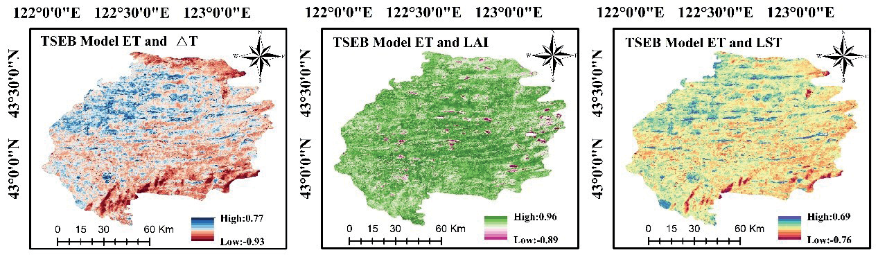
An analysis of the influencing factors revealed that distinct elements exerted varying impacts on ET across different seasons. Throughout the entire growth period, ET demonstrated a relationship with the LAI, whereas in the latter phases of vegetation development, it was primarily driven by the ΔT. Furthermore, these three driving factors were sensitive to seasonal fluctuations, contributing to the seasonal variability observed in ET. This high correlation indicated the critical importance of LAI as a parameter for precise ET estimation, which was consistent with the findings of Richard [53]. Therefore, the accurate inversion of LAI data was essential for achieving precise regional ET simulations [54].
Conclusions
This study focused on evaluating the simulation performance of the TSEB and METRIC models for complex underlying surfaces. Over a 5-year period, a remote sensing ET investigation was conducted to validate both models across diverse land types and two ecological gradients. The specific findings can be summarized as follows: The TSEB model exhibited superior fitting results in dune areas and at a regional scale when compared to the METRIC model. Conversely, the METRIC model performed the most effectively in simulating the latent heat flux in meadow areas. Generally, the METRIC model was more suitable for regions with higher vegetation indices, such as grasslands, whereas the TSEB model was superior in areas characterized by bare soil and sparse vegetation. Furthermore, the TSEB model revealed seasonal and significant spatial variations in ET for the year 2022, with lakes presenting the highest values and urban areas the lowest. ET exhibited a rapid increase during the early growth stage, reaching its zenith in August. However, during the crop harvesting process, the southern regions experienced a significant decrease in ET by early October. Regarding the comparison of model input factors, such as LAI, LST, and ΔT, and their relationships with ET, ET initially increased with LAI and then decreased, reaching its peak in August. The LST reached its highest point in May and gradually decreased from August to October. The impact of ΔT on ET was substantial, demonstrating a negative correlation in high DEM areas and a positive correlation in low DEM areas. Seasonal variations were primarily affected by LAI, ΔT, and LST, with LAI displaying a strong correlation with ET, indicating its critical role in accurately simulating regional ET. Due to significant cloud contamination issues in Landsat satellite imagery, performing ET inversion throughout the entire growing season can pose challenges. As a recommendation for future work, it is advisable to combine MODIS satellite products with Landsat satellite data by utilizing spatiotemporal adaptive fusion algorithms and the TSEB model. This approach would enable the filling of missing image data and precise estimation of evapotranspiration over multiple years across the entire study area.