

Introduction
Main in recent years, as global industrialization has accelerated, oil has been described as the “blood of industry”, serving as the world’s primary energy source and chemical raw material. With the advent of numerous industrialized sites across the globe, oil pollution has emerged as a significant concern. When petroleum pollutants exhibit slight solubility in water or complete insolubility in water, they are classified as non-aqueous phase liquids (NAPLs). A light, non-aqueous phase liquid is defined as a substance with a density less than that of water [1].The spatial distribution of LNAPL in the subsurface following leakage is challenging to anticipate due to the structural heterogeneity and inherent uncertainty of the soil. Following the leakage of Light Non-aqueous Phase Liquids (LNAPLs), the substance penetrates the subsurface under the influence of gravity, subsequently seeping into the upper part of the unconfined aquifer [2]. During the migration process, some LNAPLs become trapped within the pore space as a result of discontinuities, while others are retained on localized low-permeability features, thereby forming LNAPL aggregates [3, 4]. This results in long-term groundwater contamination that can persist for decades or even centuries, which has a detrimental impact on the surrounding human environment. Consequently, an increasing number of scholars are engaged in research on groundwater pollution by LNAPL.
The minimization of environmental damage is contingent upon the accurate and expeditious characterization of the extent of LNAPL leakage, contamination, and migration processes. However, LNAPL does not typically pass through infiltration zones in a homogeneous diffusion pattern. Rather, it migrates in discrete clusters and is highly mobile at the groundwater table [5, 6]. When LNAPL is transported vertically to a capillary zone with high water content, the capillary zone’s retention effect is enhanced [7]. When LNAPL migrates in proximity to the water table, it will not continue to migrate in a downward direction but rather will form an oil slick at the water table [8, 9]. The migration characteristics of LNAPL in aquifers are complex, and the study of LNAPL in aquifers has thus far presented a significant challenge.
Conventional techniques for monitoring leakage of non-aqueous phase liquids (LNAPL) include the use of borehole samples and groundwater monitoring wells. However, these techniques are unable to effectively monitor small leaks and provide an accurate representation of the extent of contamination and damage to the surrounding medium. Additionally, they are challenging to repeat under identical conditions and do not facilitate long-term dynamic monitoring [10, 11]. In contrast to traditional investigative techniques, Electrical Resistivity Tomography (ERT) has been employed for the monitoring of sites contaminated with liquid natural apatite (LNAPL). The resistivity signal is primarily attributable to the high resistivity of the separated-phase liquid, which impedes the flow of current through the fully saturated pore space [12]. Conversely, time-shifted geophysical methods are employed to constrain the geophysical inversion problem, thereby reducing inversion errors and facilitating the acquisition of more accurate subsurface spatial information [13, 14]. Consequently, ERT is capable of acquiring continuous subsurface resistivity data in addition to comprehensive profile information in a rapid and non-destructive manner [15].
ERT has been employed extensively to monitor the extent of contamination by LNAPLs. On the one hand, a considerable number of scholars have conducted experimental studies on the transport of LNAPLs in indoor settings. Alesse et al. [16] employed geophysical techniques, including ERT, Induced Polarization (IP), and Ground Penetrating Radar (GPR), to monitor LNAPL-contaminated sandboxes for a period exceeding 124 days. This study demonstrated the efficacy of ERT and GPR in providing complementary insights into the subsurface distribution of LNAPLs. Ali et al. [17] employed ERT to ascertain the resistivity of LNAPL contaminants, discovering that diesel fuel exhibited markedly higher resistivity than motor oil in clay soil with identical water content. Similarly, Orlando et al. [18] utilized a combination of techniques, including photo imagery, ERT, IP, and GPR, to monitor granular glass beads under saturated contamination conditions with HFE-7100 (hydrofluoroether). Reliable links were established between geophysical and physicochemical parameters of contaminated soils, thus reducing ambiguities in data interpretation. Pollock et al. [19] employed sodium chloride as a tracer in sandboxes, employing ERT and photographic imaging to ascertain the distribution of the tracer within the sandboxes. The results of the tests demonstrated that the lenticular bodies of the various sand types were not entirely homogeneous and that preferential flow paths were present. Sentenac et al. [20] conducted a study to assess the efficacy of Oxygen-Releasing Compound (ORC) in preventing the migration of LNAPL. To this end, they injected two contaminants, namely ORC and LNAPL, using ERT. The findings of the study demonstrated that the LNAPL contaminant plume was partially obstructed by the ORC barrier and that the ERT technique is an effective method for monitoring the efficacy of the barrier. Conversely, investigations have been conducted on LNAPL-contaminated sites with regard to the efficacy of LNAPL remediation through the use of ERT monitoring. This approach involves the injection of reagents into the soil substrate with the objective of stimulating the desorption and oxidation of residual hydrocarbons, as demonstrated by Ciampi et al. [21]. The results of the ERT monitoring technique demonstrated the efficacy of the intervention test, with the majority of organic pollutants undergoing decomposition. Atekwana et al. [22] employed ERT to monitor the microbial degradation of LNAPL and demonstrated that the microbial degradation process resulted in notable alterations to the contaminated environment, including significant changes in the physical properties of the rock. In the course of investigations conducted at sites contaminated with LNAPL, it is essential to take into account the microbial and geochemical contexts when significant spatial variations are observed. Ciampi et al. [23] employed ERT to track tracer migration pathways through real-time subsurface dynamics, monitoring changes in resistivity. Furthermore, the integration of groundwater sampling data facilitated the acquisition of additional insights into contaminant changes. Arato et al. [24] employed a multifaceted approach to characterize an aging LNAPL-contaminated site. The resistivity characterization was then compared with the results of the hydrocarbon contamination analysis of soil and groundwater samples. The findings indicated that elevated resistivity anomalies were markedly correlated with peaks in total organic matter and degradation by-products. Meng et al. [25] and Kaufmann et al. [26] employed ERT to examine the environmental impact of abandoned perfume factories and gas stations. Their findings revealed that ERT could effectively delineate the extent of LNAPL contamination with high spatial resolution, corroborating with borehole data and offering a cost-effective approach to remediation. Kim et al. [27] proposed the use of seismic refraction, GPR, ERT, and Complex Resistivity (CR) to map the extent of NAPL contamination. They also compared the expected contaminated area based on geophysical and soil sampling data and improved the interpretation of geophysical data at sites with NAPL contamination. Rajab et al. [28] employed Time Domain Electromagnetic Method (TEM)) and ERT to assess the extent of LNAPL contamination at the Hussein Thermal Power Station (HTPS). Their findings, based on geophysical and hydrogeological methods, indicated the presence of subsurface zones with elevated conductivity and resistivity, as well as the extent of contamination by aged LNAPL materials and industrial fluid leakage. Shao et al. [29] employed ERT in wells to monitor the resistivity change of an LNAPL-contaminated area in real-time. They then adopted a time-shift data processing method to obtain the dynamic change information of the contaminated area, which enabled them to assess the degree of LNAPL contamination quantitatively. As can be seen from the above, there is a relatively greater number of studies on LNAPL-contaminated groundwater using geophysical methods, with the majority of these based on the resistivity and migration law. Nevertheless, in order for ERT to effectively monitor the saturation distribution of LNAPL, it is essential to consider the hydrogeological conditions, given that the distribution characteristics of groundwater are particularly susceptible to change. Consequently, a comprehensive investigation into the migration process and saturation distribution of LNAPL under diverse water distribution characteristics is imperative.
In order to quantitatively study the migration process and saturation distribution of LNAPL under the specific characteristics of water distribution. In this study, the Miller Soil Box apparatus was employed in a laboratory setting to ascertain the diesel-water resistivity relationship. Furthermore, the combined use of ERT and the Miller Soil Box device enables the monitoring of diesel fuel response characteristics in a three-dimensional homogeneous sandbox under varying moisture distribution conditions, thereby establishing a foundation for the monitoring of LNAPL transport and the determination of pollution distribution.
Materials and Methods
Test Material
The test medium was primarily composed of fine sand, which was subjected to a drying and purification process to remove any impurities. The particle size of the sand samples ranged from 0.005 mm to 2 mm, with a mean particle size of 0.205 mm. The proportion of particles with a size of 0.005 mm was 5.3%, while those with a size of 0.005 to 0.075 mm accounted for 12.9%. The proportion of particles with a size of 0.075 to 0.25 mm was 38.1%, while those with a size of 0.25 to 0.5 mm accounted for 26.2%. The proportion of particles with a size of 0.5 to 2 mm was 17.5%. The mean particle size was 0.205 mm, the specific gravity was 2.68, the inhomogeneity coefficient was 30.87, the curvature coefficient was 4.78, and the predominant particle size of sandy soil particles was 0.075 mm to 0.25 mm. The coefficient of unevenness of the sand samples was found to be considerable, exhibiting a value that was significantly greater than 10.
In order to simulate the leakage behavior of LNAPL, 0# diesel fuel was employed in this experiment. 0# diesel fuel is characterized by the following properties: insolubility in water, low viscosity, a density of 0.829 g/ml, a boiling point range of 180-370ºC, and an ignition point of 220ºC. Given that the conductivity of LNAPL is 0.15 mS/cm, which demonstrates high resistivity characteristics, it is reasonable to conclude that ERT can be applied to the detection process. In light of these characteristics, 0# diesel was selected as the simulant for LNAPL pollutants in this experiment.
Test Equipment
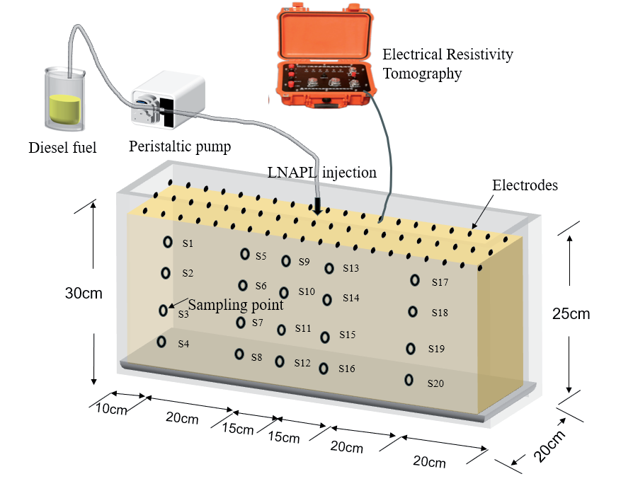
The tests were conducted in a Plexiglas box with the following dimensions: 1 m×0.2 m×0.3 m (see Fig. 1). To mitigate the impact of boundary conditions on the test outcomes, the internal edges of the sandbox were coated with petroleum jelly [30] Once the sandbox was filled, copper electrodes were arranged on the surface of the medium. Each electrode had a length of 8 cm, a diameter of 0.5 cm, and an electrode spacing of 4 cm. Each row was equipped with 20 electrodes, and a total of 3 rows of electrodes were arranged in accordance with the optimal distance between electrodes, as previously described [31]. Each electrode was connected to the Electrical Resistivity Tomography apparatus via a multi-core cable. The LNAPL was introduced to the system via the locations designated as “sampling points” in Fig. 1, and the rate and volume of leakage were precisely controlled by a peristaltic pump.
Test Methods
Test Medium Filling
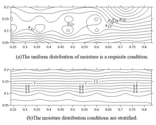
In the sandbox test, two kinds of sandy soils with moisture distribution characteristics were filled: uniform moisture distribution sandy soil and stratified moisture distribution sandy soil. The conditions of moisture distribution characteristics of the two sandy soils are shown in Fig. 2. The stratified moisture distribution of sandy soil is characterized by the fact that the moisture content of the upper sandy soil in the sandbox is higher than that of the underlying sandy soil, with a range of 5.8% to 8.2% and an average moisture content of 7%. In contrast, uniform moisture distribution in sandy soil means that the sandy soil inside the sandbox has the same moisture content, which ranges from 9% to 9.3%. After filling, the moisture content was tested and verified using a portable soil moisture meter. Since the test time did not exceed 24 hours and the water content of the sandy soil was low, the effect of vertical migration of free water in the sandy soil under gravity was ignored in this test.
Test Procedure
The initial state (background) was recorded on three occasions with a resistivity meter prior to the injection of LNAPL. The background measurements were performed using a dipole device with the objective of characterizing the resistivity conditions in the uncontaminated state. The mean of the background measurements was employed as a reference point for the generation of disparate delayed images during the subsequent migration of the LNAPL.
Real-time measurements of the high-density resistivity method were maintained throughout the course of the experiment to monitor the continuous movement of LNAPL. The LNAPL was injected using a peristaltic pump at 2 rpm in a total volume of 1000 mL for 180 min at an average rate of 5.55 mL/min, and ERT data were collected every 30 min until the end of the LNAPL injection. Each data collection period lasted 1.5 min. During this time, the actual volume of LNAPL injected was 8.3 mL. Given the total injection time of 180 min and the total injected volume of 1000 mL, the movement of LNAPL could be approximated to be negligible in the short period of ERT data collection.
Precision Analysis
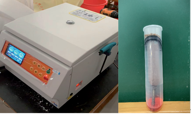
The stratified samples were obtained immediately following the conclusion of the tests conducted using the ERT. Following the sampling procedure, the specimens were placed in a constant temperature box at 25°C in order to conduct a precision test. The sandbox was configured with three groups of profiles for sampling, designated P1 to P3. Each group of profiles comprised 20 sampling points, labeled S1 to S20, with the sampling points in the same layer spaced 15 cm apart and an interval of 10 cm between layers, for a total of 60 sampling points. The location of the sampling points is illustrated in Fig. 1. In the preceding residual volumetric water content test, it was established that when the medium is sandy soil, the residual volumetric water content in the sandy soil is less than that in the soil subjected to centrifuge centrifugal force. Consequently, the homemade centrifugal tube device, illustrated in Fig. 3, was employed to carry out centrifugation on the sandy soil from the sandbox test sampling.
Data Processing
A total of 64 test electrodes were accessed in this test, and the selected equipment operated in the multi-channel time-varying automatic measurement-scanning mode. Once the resistance data acquisition was complete, the visual resistivity data were inverted to real resistivity data using the least squares inversion method via the ReslPy software. Subsequently, the resistivity data were imported into the Surfer software, which was used to generate an image of the resistivity distribution within the sandbox. The same Surfer software was employed to construct the LNAPL saturation distribution graphs. Additionally, the LNAPL saturation distribution was plotted using the Surfer software.
Results and Discussion
Relationship between LNAPL Content and Resistivity
In this paper, we combined the previous experience of using the Miller Soil Box to measure the resistivity of the medium [32-35] with the use of the homemade Miller Soil Box as the measuring device for the experiments. The latter was made of Plexiglas in the form of a rectangle with dimensions of 21 cm in length. The device was 5 cm in width and 5 cm in height, and the electrodes for measuring current at the two ends were made of pure copper and had the same dimensions as those of the rectangle. M N was connected to a voltmeter, and the two ends of the device were connected to the positive and negative poles of the direct current (DC) power supply, as illustrated in Fig. 4. The current-measuring electrodes at both ends were constructed from pure copper with the same cross-sectional dimensions as the rectangle. The MN was connected to a voltmeter, and both ends of the device were connected to the positive and negative poles of the DC power supply, as illustrated in Fig. 4. The sand samples utilized in the experiment were combined with water and oil in varying proportions, and the resistivity data under distinct water and oil concentrations were obtained through resistivity measurements on these mixed sand samples. The relationship between resistivity and water content for sandy soils with varying oil content is illustrated in Fig. 5.
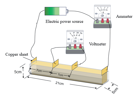
Fig. 5.
Illustrates the resistivity versus water content curves for sandy soils with varying oil content conditions.
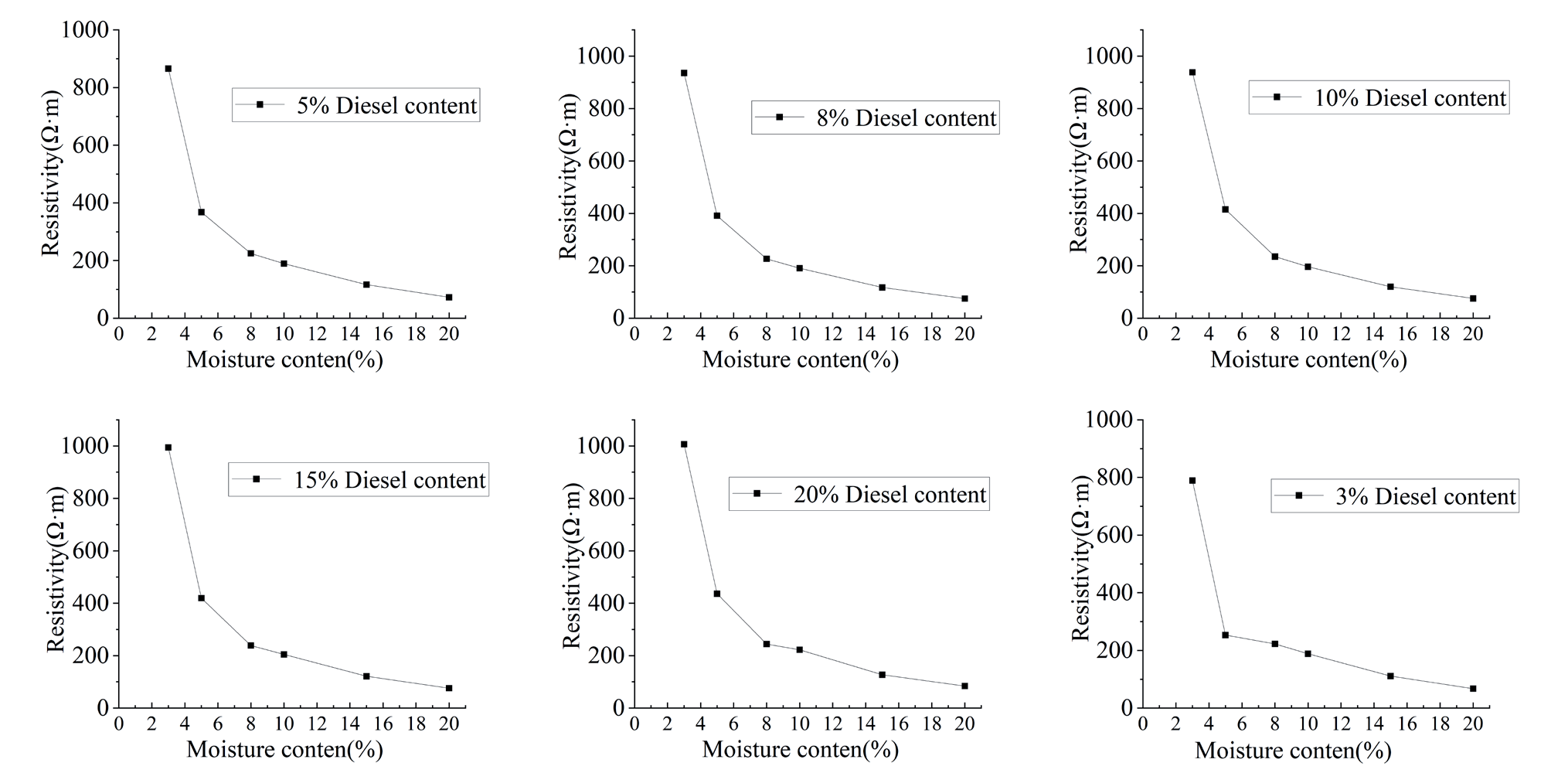
The results presented in Fig. 5 demonstrate that the resistivity exhibits a decreasing trend with increasing water content at a constant oil content. Conversely, the resistivity demonstrates a slight increasing trend with increasing oil content at a constant water content. It is evident that the resistivity is significantly influenced by the water content, whereas the oil content exerts a comparatively lesser effect on the resistivity.
A LogNormal 2D function was employed to fit a nonlinear surface to the data pertaining to water content, oil content, and corresponding resistivity. The three-dimensional fitting plots of the water content, oil content, and resistivity are presented in Fig. 6. As can be observed in Fig. 6, the fitting results are satisfactory, and the fitting Equation is as follows:
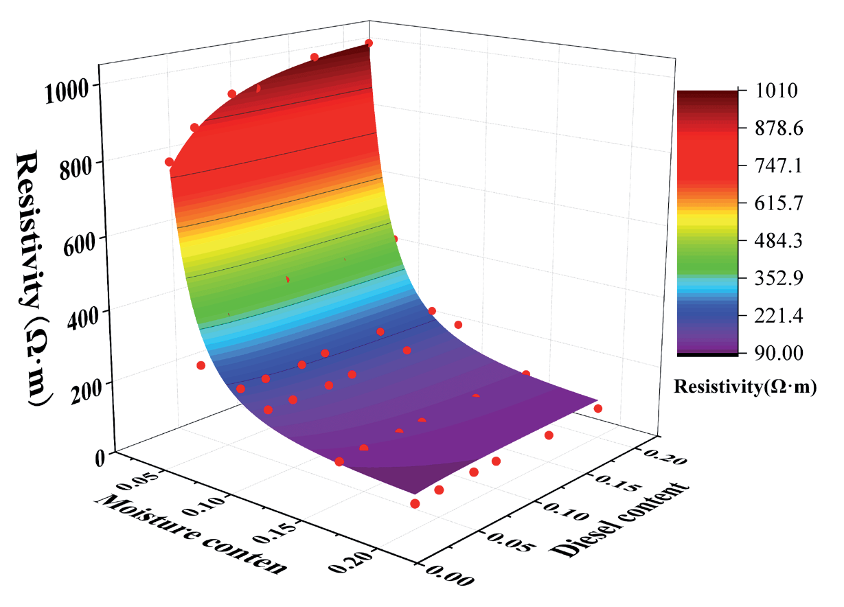
Where, x: Water content (%), y: Oil content (%), z: Resistivity (Ω·m), z0 = 37.00783, B = -16053.33903, C = 1.84357e-5, D = 2.04502, E = 51.3197, F = 0.30925, G = 3.09311, H = 656135.45966.
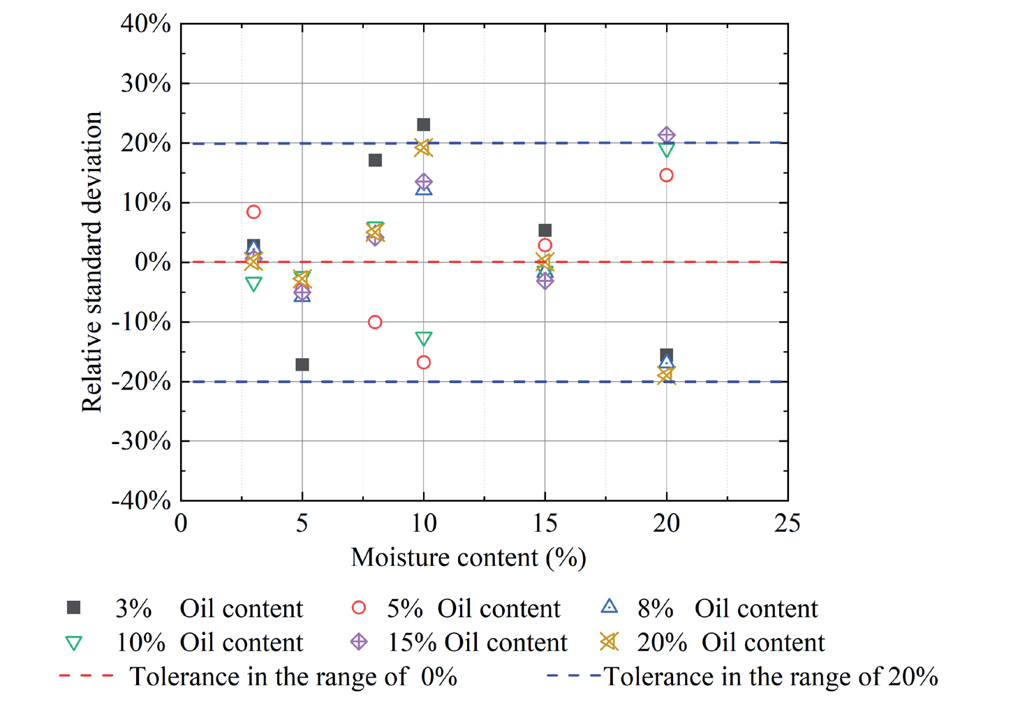
The oil and water contents of the Miller Soil Box are substituted into Equation (1) in order to calculate the resistivity, and a relative error analysis is carried out using the resistivity measured in the test, as illustrated in Fig. 7. The results demonstrate that the relative error is maintained at a level of 20% or less. Accordingly, Equation (1) is applied to the three-dimensional sandbox (uniformly filled with sand, with reasonable assumptions), and the resistivity value and water content can be obtained from the three-dimensional sandbox oil content, thus enabling the calculation of the saturation degree of LNAPL.
Characterization of LNAPL Leakage Processes under Different Moisture Distribution Characteristics
Resistivity Inversion Results Depict the LNAPL Migration Process
The transport diffusion of LNAPL in sandy soils can be divided into the redistribution stage of LNAPL under stratified moisture distribution characteristics and uniform moisture distribution characteristics. In this section, the resistivity inversion results of LNAPL under stratified moisture distribution characteristics and uniform moisture distribution characteristics are analyzed, respectively, to study the migration pattern of LNAPL in these two stages.
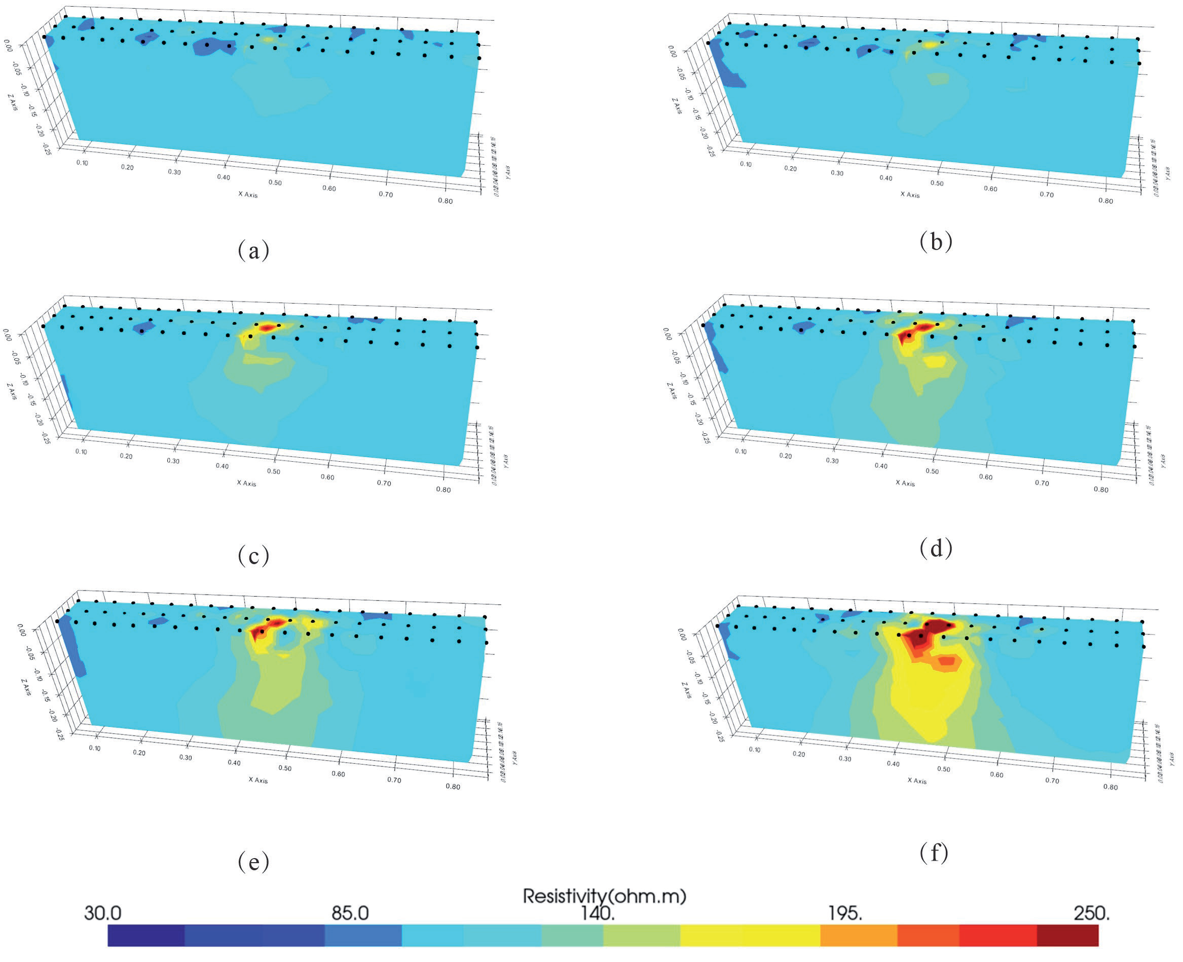
1) Results of resistivity inversion and analysis of LNAPL under stratified moisture distribution characteristics. Fig. 8 shows the results of resistivity changes at different moments during LNAPL leakage under stratified moisture distribution characteristics. The average values of sandbox resistivity are 95 Ω·m when LNAPL is not leaking, respectively, and due to the non-ideal homogeneity of the soil body, the resistivity in the local area of the sandbox is lower than 85 Ω·m. Fig. 8a) shows that when t1 = 30 min, only the resistivity of the central region increases, which is due to the transport and diffusion of LNAPL in the longitudinal and horizontal directions of the sandy soil under the effects of gravity, capillary force, and infiltration pressure. From t2 = 60 min to t3 = 90 min, with the continuous injection of LNAPL, the resistivity value of the central area increased, and the area of the contaminated area expanded because the LNAPL migrated mainly vertically under the effect of gravity. From t3 = 90 min (Fig. 8c)) to t4 = 120 min (Fig. 8f)), the LNAPL migrated laterally into the low water content area. Compared with the high water-content sand layer, the low water-content sand has a larger porosity, and it is easier for LNAPL to penetrate into the pore space, which increases the mobility of LNAPL and results in lateral migration. At t4 = 120 min (Fig. 8d)), the images were not significantly different from those at t5 = 150 min, but the resistivity of the sandy soils in the contaminated zone gradually increased, which was attributed to the gradual saturation of the soils with LNAPL due to the continuous dosing of LNAPL. At t6 = 180 min, the resistivity at the leakage port reached 250 Ω·m, which was attributed to the LNAPL saturation at the leakage port due to the continuous feeding of LNAPL, and there was a more significant lateral transport diffusion phenomenon in the subsoil, which was in the shape of a “volcano”, reflecting the fact that the LNAPL in the horizontal direction was not saturated with LNAPL. Horizontally, the LNAPL gradually spread from the high concentration area to the low concentration area until the concentration tended to follow a uniform transport law.
Fig. 8.
The resistivity versus time as leakage of liquid nitrogen-absorbing particles (LNAPL) occurs under conditions of stratified moisture distribution characterization.
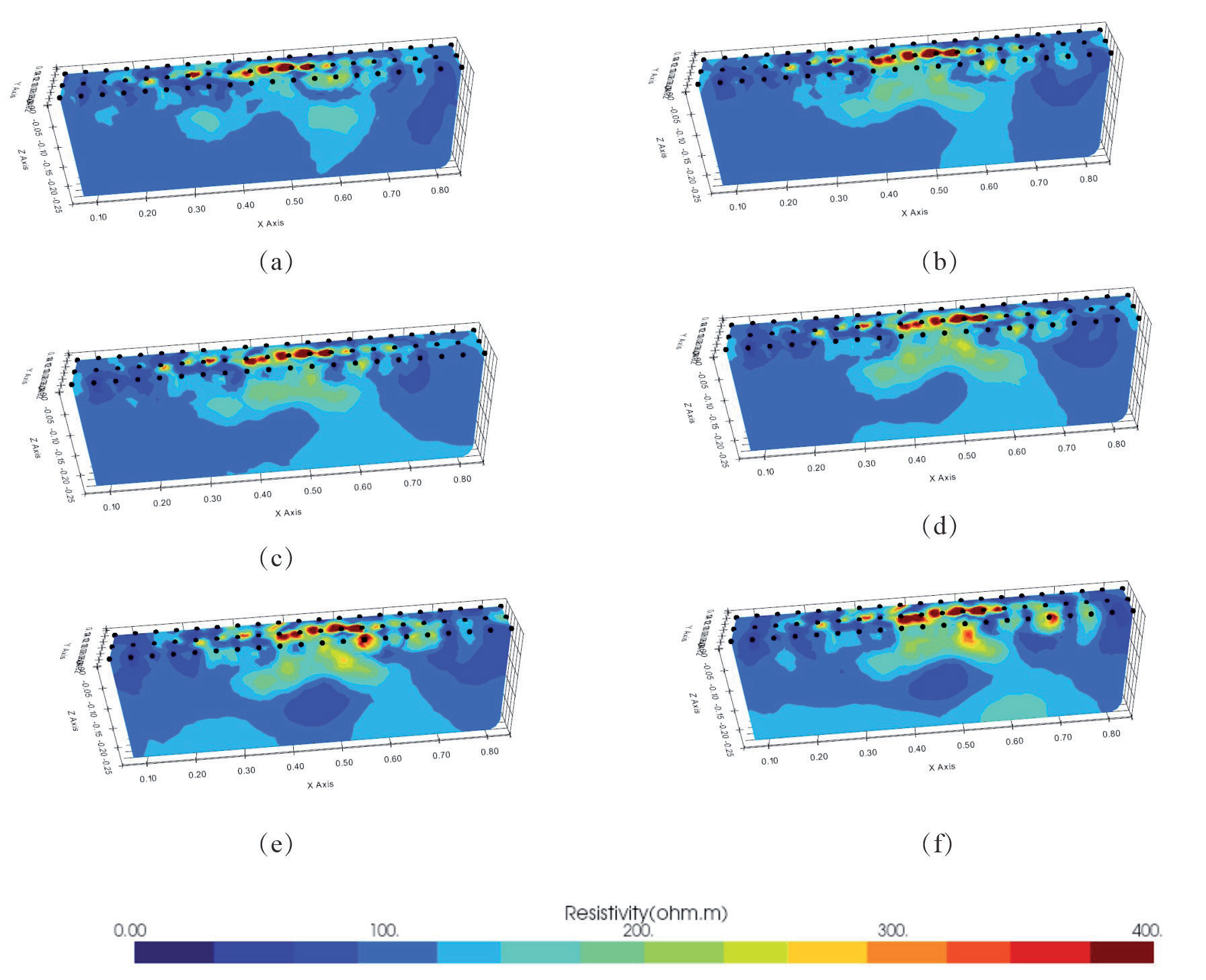
2) Results of resistivity inversion and analysis of LNAPL under uniform moisture content. Fig. 9 shows the plot of sand resistivity with time under the characteristic condition of uniform moisture distribution. The average value of sandbox resistivity is 100 Ω·m when LNAPL is not leaking, and due to the non-ideal homogeneity of soil, the resistivity in the local area of the sandbox is lower than 90 Ω·m. The resistivity of the sandbox is less than 90 Ω·m when LNAPL is not leaking. From Fig. 8, it can be observed that as LNAPL infiltrates from the leakage port area, the resistivity value continues to increase from 100 Ω·m to 400 Ω·m, reflecting the presence of LNAPL as a high-resistance body in the medium.
In the early stage of leakage, LNAPL mainly migrated vertically, and after 30 min, LNAPL migrated to the bottom of the sandbox. The image color of this area showed light blue, the resistivity value changed less, and its range was between 120 and 150 Ω·m, which indicated that the resistivity monitoring could clearly depict the smaller area of the contaminated area under the condition of low concentration. The reason was analyzed as the vertical migration of LNAPL under the effect of gravity; the gravity of LNAPL was much greater than the capillary force, and the vertical diffusion was greater than the lateral diffusion.
As the quantity of LNAPL injection increases, the extent of the contaminated area expands, accompanied by an increase in resistivity value. The lower portion of the contaminated area exhibits a green hue, the central region displays a yellowish tint, and the resistivity value ranges from 150 to 250 Ω·m. The dominant channel is observed on the right side of the sandbox (x = 0.6 m), and lateral diffusion occurs at the bottom of the sandbox. As a consequence of the sustained injection of LNAPL, the water within the pore space was displaced, resulting in the formation of a free-flowing dominant channel for LNAPL. Upon reaching the bottom of the sandbox via the dominant channel, lateral migration of the LNAPL occurred. At t = 150 min, a decrease in resistivity value was observed in the middle of the sandbox (x = 0.45 m, z = 0.15 m). The resistivity value decreased from 100 Ω·m to 80 Ω·m, indicating that following the injection of LNAPL into the medium, the LNAPL in the upper pore space was replaced by the action of gravity, and the LNAPL in the lower pore space was displaced. This indicates that following the injection of LNAPL into the medium, the upper LNAPL is displaced by gravity and the lower LNAPL, and the water in the pore space is displaced, resulting in the formation of a region with a reduced resistivity value. As the LNAPL injection continued, the contaminated area expanded, accompanied by an increase in resistivity value. This resulted in the formation of a C-shaped distribution, with a low resistivity value in the center and a high resistivity value in the surrounding area. This demonstrates that the pollutants in LNAPL are continuously replacing the pore water transport law, influenced by capillary force and gravity.
The Resistivity at Various Points along the Migration Process Can Be Used to Illustrate the Movement of the LNAPL
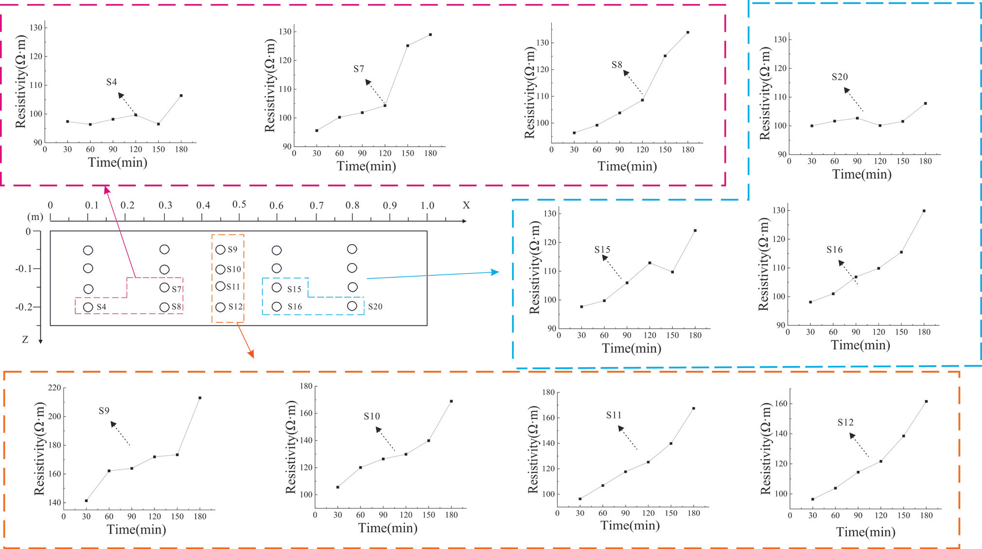
Fig. 10 illustrates the resistivity change curve of fixed points in profile 1. As the leakage time of LNAPL increases, the resistivity of S9, S10, S11, and S12 significantly rises, exceeding 60 Ω·m. This phenomenon can be attributed to the location of these points at the base of the leakage mouth. The continuous leakage of LNAPL is primarily a vertical migration process that results in leakage. The resistivity change of points situated below the leakage port is more pronounced than that of other points. In this regard, measurement point S9 reaches a stable stage after 60 min, and the resistivity rises abruptly after 150 min. The reason for this is that the potential is initially polluted by LNAPL leakage. Over time, a portion of the LNAPL in the sand and soil is transported to the surrounding area in the form of liquid, with the rate of transport subsequently decreasing. This results in the LNAPL gathering at the point, which in turn leads to an increase in the resistivity of S7. The resistivity of S7, S8, S15, and S16 continued to increase over time, indicating that with the increase in the amount of LNAPL injection, the contaminated area continues to expand, and the resistivity value increases accordingly. The resistivity changes observed in S4 and S20 are relatively smooth. At t = 150 min, however, the resistivity of these points began to increase. This can be attributed to the fact that the points are situated at a greater distance from the leakage port, with the LNAPL concentration in the sand and soil being greater than that at the leakage port. The aggregation of the LNAPL in the point results in an overall increase in resistivity. The reason for this is that the point is situated at a considerable distance from the leakage outlet. Consequently, the resistivity change is relatively minor when the LNAPL is not transported to this location. However, following the arrival of the LNAPL front, a notable increase in resistivity is observed.
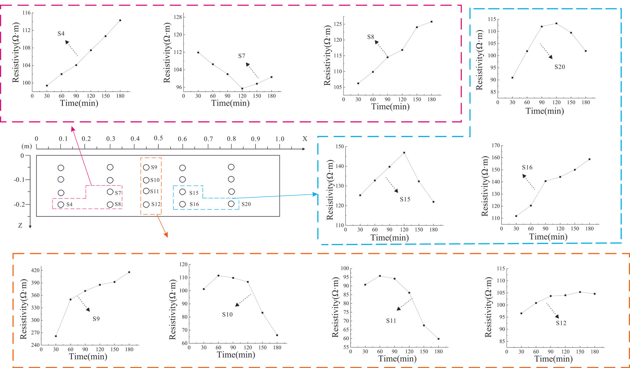
Fig. 11 illustrates the resistivity curves over time at various points beneath a uniform moisture distribution. As illustrated in Fig. 11, the resistivity of S4, S8, S9, S12, and S16 exhibited a notable increase over time. This suggests that with the injection of increasing amounts of LNAPL, the extent of contamination also expanded, accompanied by a corresponding rise in resistivity. The resistivity value of point S7 demonstrates a pattern of initial decline and subsequent increase. This can be attributed to the replacement of pore water by LNAPL at point S7, which causes a continuous decrease in resistivity. As the LNAPL injection continues, the LNAPL begins to replace the pore water at point S7, resulting in a corresponding increase in resistivity. At t = 90 min, points S10 and S11 exhibit an inflection point in resistivity. As time progresses, the resistivity of these points decreases significantly, exceeding a 30 Ω·m reduction. This phenomenon can be attributed to the displacement of LNAPL towards the center of the pore water, which results in a notable decline in resistivity. The resistivity of points S15 and S20 demonstrates a pattern of initial increase followed by subsequent decrease. This is attributed to the continuous injection of LNAPL, which migrates to the right side of the sandbox, thereby reducing the LNAPL content at this point. Consequently, the resistivity pattern exhibits an initial increase followed by a subsequent decrease.
The Process of Migration is Exemplified by the Phenomenon of LNAPL Saturation
By comparing the plots, the time-shifted ERT data inversion method can provide an approximate localization of the plume position and describe the temporal evolution of its general shape. While direct inversion can provide an approximate characterization of the LNAPL morphology, it may also result in the loss of information regarding the plume’s intricate details. In order to assist with constraining the coupled inversion, the inverted resistivity image data were employed as known a priori information. The LNAPL content was calculated by substituting the inverted resistivity data and water content into Equation (1), which was used to determine the LNAPL saturation. Fig. 12 depicts the estimated distribution of the LNAPL, obtained through the fitting of Equation.
The plot of estimated LNAPL saturation from t3 to t6 reveals an increasing trend in the saturation of the LNAPL within the sandbox, while the saturation in the upper medium exhibits significant fluctuations, and that in the lower medium remains relatively low. As illustrated in Fig. 12, the LNAPL initially migrated vertically downward, reaching an infiltration depth of 20 cm at 90 min. Subsequently, it was transported horizontally under the influence of capillary forces, exhibiting a distinct ‘volcano’-shaped migration pattern. This observed behavior was found to be consistent with the reference figure.
In comparison to the inversion map (Fig. 8), direct inversion enables a preliminary reconstruction of the distribution of LNAPL saturation. However, the direct inversion results indicate that LNAPL clusters at the top (Fig. 8e) and f)), which differs from the estimated distribution (Fig. 12e) and f)). This is primarily due to the fact that medium variability (e.g., local variations in sand moisture content) may result in minor resistivity fluctuations. In such instances, the resistivity generated by direct inversion is unable to delineate the intricate structure of the LNAPL contamination plume accurately. Consequently, the inversion outcomes (resistivity) are transformed into hydrological states under the limiting condition of incorporating medium moisture content, thereby facilitating a more comprehensive characterization of the LNAPL contamination plume’s distribution.
Fig. 12.
Distribution of LNAPL saturation under conditions characterized by stratified moisture distribution.
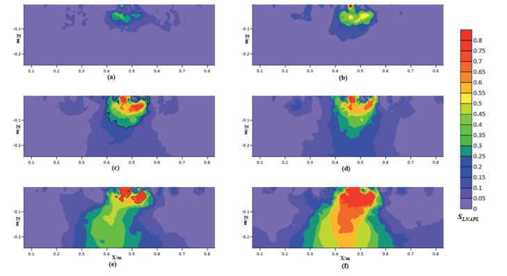
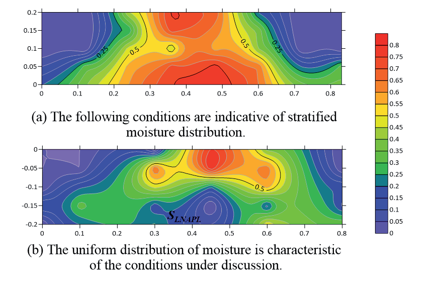
Fig. 13 illustrates the LNAPL saturation at various points in time. The migration of the LNAPL is predominantly influenced by gravity, reaching the base of the sandbox where lateral diffusion occurs. The LNAPL saturation in the central region is 0.5, which aligns with the findings of the direct inversion analysis.
Precision Analysis
In this experiment, the medium was subjected to centrifugation at 4800 rpm for a period of two hours under conditions of water saturation and LNAPL equilibrium. The residual water content by volume and the residual LNAPL rate by volume were subsequently calculated to be 1.52% and 1.36%, respectively. The residual water content and LNAPL rate in sandy soil are within the error range. Based on a review of the literature, it can be concluded that a centrifugation time of 100 min is sufficient to meet the test requirements when determining the residual water content and LNAPL rate. Accordingly, the test was conducted using a centrifuge at a rotation speed of 4800 rpm and a centrifugation time of 2 hours to fulfill the necessary requirements. Fig. 14 depicts the graph of LNAPL saturation, calculated through the centrifugation of samples. A comparison of Fig. 12f) and Fig. 14a) with Fig. 1f) and Fig. 14b) reveals that the calculated LNAPL saturation distribution is consistent with the LNAPL saturation distribution after centrifugation in the centrifuge, thereby verifying the correctness of the formula for calculating LNAPL saturation distribution.
This study employs the high-density resistivity method to monitor the transport pattern and saturation distribution of LNAPL under diverse conditions of moisture distribution characteristics. The study demonstrates that the transport pattern of LNAPL under disparate conditions of moisture distribution characteristics is relatively intricate. However, it is feasible to characterize the transport pattern of LNAPL through the geophysical method of ERT. Additionally, it was observed that when specific variables do not influence the outcomes, the oil and water content, as well as the saturation distribution of LNAPL in sandy soils, exhibit a functional relationship with resistivity. This functional relationship allows for the quantification of the LNAPL saturation distribution in sandy soils through the measurement of water content as a function of resistivity.
The results of resistivity measurements in sandbox sandy soils demonstrated that under conditions of stratified moisture distribution, ERT was capable of monitoring the migration process of LNAPL, which diffused towards areas of low saturation. However, under conditions of uniform moisture distribution, the sandy soils exhibited the phenomenon of “LNAPL replacement of pore water” and “dominant channel”. The phenomenon of the “dominant channel” occurs in sandy soils under conditions of uniform water distribution characteristics.
Fig. 13.
Distribution of LNAPL saturation under conditions characterized by uniform moisture distribution.
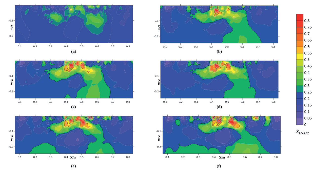
Fig. 14.
A calculation of the distribution of saturated LNAPL samples following the processes of sampling and centrifugation is presented.
The immiscibility of oil and water in sandy soil results in the two liquids coexisting in the porous medium, which is composed of particles of sandy soil with highly inconsistent geometrical shapes and sizes. The formation of a complex spatial network determines the microgeometric structure of the pore medium and the surface properties to be extremely inhomogeneous. The high resistivity plume provides a clear illustration of the spatial and temporal migration paths of LNAPL under experimental conditions. This is in alignment with the findings of the error analysis and validation and serves to confirm the potential of ERT imagery for monitoring LNAPL transport and the extent of contamination.
Conclusions
In this study, a systematic measurement and analysis system based on ERT was employed to obtain images of LNAPL saturation distribution under homogeneous conditions with varying moisture distribution characteristics. These images clearly reflected the effectiveness of ERT in monitoring pollutant transport and describing the transport process of LNAPL. The following conclusions were drawn:
(1) The relationship between different oil and water content and resistivity was measured using the Miller Soil Box. A relationship equation was established between the three variables. When the oil content is held constant, the resistivity exhibits a pronounced variation with the water content, whereas the resistivity displays less fluctuation with the oil content when the water content is maintained at a constant level.
(2) The transport process of LNAPL pollutants is primarily influenced by gravity and capillary forces. In the longitudinal direction, the transport of LNAPL pollutants is predominantly governed by gravity and capillary forces. Conversely, in the transverse direction, capillary forces play a dominant role.
(3) In the context of stratified moisture distribution characteristics, the vertical transport of LNAPL was observed to occur under the influence of gravity and capillary forces. The longitudinal movement was found to be more pronounced than the transverse movement, with a transport time of 90 min to the bottom of the sandbox. Upon reaching the bottom of the sandbox, the transverse transport rate of LNAPL was observed to exceed the longitudinal rate. This suggests that LNAPL accumulates at the bottom of the sandbox and then spreads to both sides, forming a volcano-like shape.
(4) In accordance with the conditions of uniform water distribution characteristics, the vertical rate of LNAPL exhibited a gradual increase, reaching the bottom of the sandbox within a 30-min timeframe. In the context of LNAPL transport within a single homogeneous medium, the prevailing transport law is subject to influence from water-oil substitution. This, in turn, gives rise to the migration of free water within the medium, which ultimately results in the formation of a dominant channel where LNAPL is relatively free. Upon reaching the bottom of the sandbox, the transverse transport rate of LNAPL is observed to exceed that of the longitudinal rate. This indicates that LNAPL accumulates at the bottom of the sandbox and subsequently spreads to the two sides, thereby exhibiting a “C” shaped distribution pattern.
(5) The relationship between resistivity and LNAPL and water content was established by the Miller Soil Box. The three-dimensional sandbox inversion resistivity data were then substituted into the established formula to estimate the distribution of LNAPL saturation in sandy soil. The accuracy of LNAPL saturation was verified by centrifugal test, which is a feasible method to study the relationship between resistivity and LNAPL saturation.
The test results are of practical significance for understanding the transport mechanism and distribution characteristics of LNAPL pollutants, as well as for determining the extent and degree of LNAPL pollution, thus enabling the formulation of a reasonable and feasible pollution control program.

