

Introduction
Over the last century, there has been remarkable economic growth and technological advancement that has significantly improved human well-being. However, this progress has also brought about environmental challenges, particularly concerning greenhouse gas (GHG) emissions [1, 2]. These emissions predominantly stem from human activities such as the widespread use of fossil fuels in sectors like electricity generation, agriculture, and transportation [3-5]. While economic growth and technological developments have positively impacted human life, the adverse environmental effects of heavy reliance on fossil fuels have become evident, underscoring the urgent need for sustainable and environmentally friendly alternatives in these critical sectors.
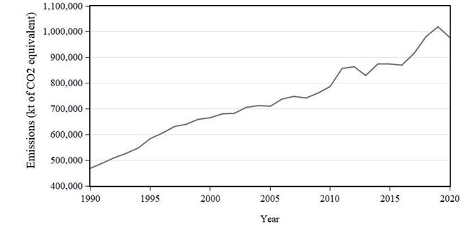
Fig. 1.
Total greenhouse gas emissions in Indonesia, 1990-2020. Source: World Development Indicators [27].
Greenhouse gas emissions have profound negative impacts on both the environment and human health [6- 8]. One of the most significant consequences is global warming, leading to climate change phenomena such as rising temperatures, melting polar ice caps, and more frequent and severe weather events like hurricanes, droughts, and floods. These changes disrupt ecosystems, threaten biodiversity, and exacerbate natural disasters, resulting in significant economic losses and decreased human welfare [9-12]. Additionally, GHG emissions contribute to air pollution, which poses serious health risks, including respiratory diseases [13-15] and cardiovascular problems [16, 17]. Moreover, the acidification of oceans due to increased carbon dioxide absorption leads to detrimental effects on marine life and ecosystems [18, 19]. Furthermore, the socio-economic impacts of climate change disproportionately affect vulnerable communities [20, 21], exacerbating inequalities and potentially leading to conflicts over scarce resources like water and arable land. Hence, the negative impacts of GHG emissions highlight the urgent need for concerted global action to mitigate climate change and transition to sustainable, low-carbon alternatives [22, 23].
The Sustainable Development Goals (SDGs) play a crucial role in reducing greenhouse gas emissions and enhancing environmental quality through their comprehensive framework addressing various facets of sustainable development. SDG 13 specifically focuses on climate action, urging nations to take immediate measures to combat climate change and its impacts, including reducing carbon emissions and adopting renewable energy sources [24]. Additionally, several other SDGs, such as SDG 7 (Affordable and Clean Energy) and SDG 12 (Responsible Consumption and Production), contribute indirectly to mitigating greenhouse gas emissions by promoting the use of clean energy technologies and sustainable consumption and production patterns. Furthermore, SDGs related to environmental protection and conservation, such as SDG 6 (Clean Water and Sanitation) and SDG 15 (Life on Land), aim to preserve ecosystems and natural resources, which can help absorb carbon dioxide and mitigate climate change. By aligning policies, investments, and actions with the SDGs, countries can foster sustainable development pathways that simultaneously reduce greenhouse gas emissions and improve environmental quality, thereby contributing to a more sustainable and resilient future for all.
According to [25], Southeast Asia emerges as one of the most vulnerable regions to the impacts of climate change due to its geographical location, extensive coastlines, and reliance on climate-sensitive sectors such as agriculture and fisheries. Consequently, it is imperative for countries within this region to adapt their policies and strategies to effectively cope with the anticipated risks of climate change [25]. Indonesia, being one of the largest countries in Southeast Asia, faces significant challenges in this regard, exacerbated by its status as one of the top emitters of GHGs in the region [26]. Data from the World Development Indicators [27] reports that total GHG emissions in 2020 were approximately 976.5 thousand kilotons of CO2 equivalent (Fig. 1). Compared to 2016, GHG gas emissions in 2020 increased by approximately 12.2% [27].
Several factors contribute to Indonesia's high emissions profile, including its heavy reliance on coal for electricity generation, deforestation activities, particularly for palm oil and timber production, and rapid industrialization and urbanization processes. The country's vast peatlands, when drained or burned for agricultural purposes, release substantial amounts of carbon dioxide (CO2) into the atmosphere. Additionally, Indonesia's agricultural practices, such as rice cultivation and livestock farming, also contribute to methane emissions [28-30]. Addressing Indonesia's status as a top emitter of GHGs requires comprehensive and coordinated efforts, including transitioning towards renewable energy sources, implementing sustainable land-use practices, and enhancing climate resilience across various sectors. Such actions not only mitigate Indonesia's contribution to global climate change but also bolster the country's capacity to adapt to its adverse impacts, ensuring a more sustainable and resilient future for its people and ecosystems.
According to [31], the livestock sector contributes significantly to global GHG emissions. The livestock sector seeks large portions of land for the rearing of animals, which leads to deforestation [32]. The Food and Agricultural Organization [33] stated that approximately 14.5% of anthropogenic GHG emissions originate from livestock supply chains. This amounts to around 7.1 gigatons (GT) of CO2 equivalent per annum [33]. The main livestock contributors to GHG emissions are from the production of animal feed and methane (CH4) from animal digestion [33, 34]. In the context of Indonesia, there is a projected increase in meat consumption from 63.60 grams to 3.36 kg per person by 2024, driven by factors such as education, income, and shifting consumer attitudes [35]. This rise in meat consumption poses significant environmental challenges, particularly concerning methane emissions, as each cattle in East Java, Indonesia's largest producer region with 4.9 million cattle, 301,000 dairy cows, and 22,900 buffaloes, emits an estimated 80–110 kg/year of methane gas [34]. Utilizing the ARIMA model, projections suggest a concerning 17% increase in GHG emissions from cattle by 2026 [34]. Therefore, there is a need for sustainable practices and policy interventions to mitigate the environmental impact of Indonesia's increasing meat industry while meeting the growing demand for animal-derived protein.
Despite extensive research on the drivers of GHG emissions globally, there remains a notable gap in understanding the specific interplay between fossil fuel consumption, meat production, forest cover, and GHG emissions in Indonesia. This gap hampers the formulation of targeted policies and interventions essential for mitigating emissions effectively in this context. Many studies have assessed the factors that influence GHG emissions; see [2, 36-52]. However, few studies have examined the impact of fossil fuel consumption, meat production, and forest cover on GHG emissions in Indonesia using a time-series econometric approach. Understanding the interplay between fossil fuel consumption, meat production, and forest cover is crucial for effectively addressing GHG emissions in Indonesia, as these factors represent significant contributors to the country's overall emissions profile. By conducting comprehensive studies on their impacts, policymakers can develop targeted strategies to mitigate emissions and promote sustainable development in alignment with Indonesia's climate goals and commitments.
Therefore, this study aims to investigate the relationship between fossil fuel, meat production, and forest cover on GHG emissions in Indonesia for the period 1990 to 2020. By employing the autoregressive distributed lag (ARDL) bounds testing approach to cointegration, it seeks to assess both short and long-run relationships among these variables. Understanding these relationships is crucial for informing evidence-based policies and interventions to effectively mitigate GHG emissions in Indonesia, thereby promoting environmental sustainability and contributing to global efforts to combat climate change.
Materials and Method
Model Specification
This study examines the impact of fossil fuel consumption, meat production, and forests on greenhouse gas emissions (GHG) emissions in Indonesia. To study the determinants of GHG emissions in Indonesia, the following model is specified:
Where GHGt denotes total greenhouse gas emissions, measured in kilotons (kt). Fossilt represents fossil fuel in kilowatt-hours (kWh). Meatt represents total meat production, which is measured in metric tons, and Forestt is the forest cover measured in square kilometers (sq. km). Epsilon (εt) is a white noise error term, and ln is the natural logarithm. α0 is the model intercept term, and α1 - α3 are parameters to be estimated for the respective determinants of GHG emissions.
Empirical Analysis
Stationarity
In time-series analysis, it's essential to perform a unit root test to evaluate whether the underlying data is stationary. Stationarity is crucial because regression analysis with time-series data relies on the assumption that certain statistical properties such as mean, variance, and covariance remain constant over time [53]. Stationarity, as described by [54] and [53], means that the statistical characteristics of a time-series remain stable over time. [55] highlight that many macroeconomic variables exhibit persistent trends without reverting to a fixed mean, making them nonstationary. This concept is vital in empirical research with time-series data because using nonstationary series in regression analysis can lead to spurious regression [55, 56]. Spurious regression can produce misleading results, suggesting significant relationships between variables that may not genuinely exist. Such misleading outcomes can lead to incorrect conclusions and, if utilized for policy decisions, may result in ineffective recommendations. Therefore, determining the integration order for each time-series used in regression analysis is crucial to avoid drawing inaccurate conclusions and making flawed policy recommendations. Therefore, the stationarity of the variables is investigated using the Augmented Dickey-Fuller (ADF) [57] and Phillips-Perron (PP) [58] tests for unit roots.
Cointegration and Error-Correction Mechanism
As previously mentioned, applying OLS or similar techniques to nonstationary time-series data can produce spurious results. One way to address this issue is by differencing the data to induce stationarity, but this approach risks overlooking important long-term relationships present in the original variables [53]. Despite short-run deviations from equilibrium, [55] emphasize that two or more variables may establish a long-run equilibrium relationship. Moreover, [59] states that if a set of time-series data exhibits an equilibrium relationship, they cannot move independently, indicating cointegration. Cointegration analysis helps identify long-run equilibrium relationships among nonstationary variables, as any short-run deviations are expected to dissipate over time, ultimately reaching long-run equilibrium.
Various methods exist for examining the presence of a long-run relationship among variables. [60] introduced a two-step residual-based technique for testing cointegration among nonstationary variables, while [61] developed a method for testing cointegration in multiple-equation models using Maximum Likelihood Estimation (MLE). However, both approaches have limitations, with the Engle-Granger method unable to identify all potential cointegrating relationships and the Johansen and Juselius method being overly restrictive by explicitly requiring all series to be integrated at the same order, 1.
This study adopts the ARDL bounds testing approach to cointegration proposed by [62] due to its less restrictive nature. Unlike other methods, the ARDL approach does not require all series to be integrated in the same order but can handle mixed orders of integration. Additionally, it is effective in small sample sizes and can simultaneously estimate the short- and long-run parameters of the model. The ARDL bounds testing approach begins by specifying a conditional error-correction model (ECM) as outlined in equation (2) as follows:
(2)
All of the variables in equation (2) are defined previously. Delta (Δ) is the difference operator, α0 is the intercept term, λ1 - λ4 are long-run parameter estimates, and β1 - β4 are the short-run parameter estimates for the determinants of GHG emissions in Indonesia. Once the conditional ECM is specified, the bounds test becomes crucial in assessing the presence of cointegration among the variables. This entails using an F-test to evaluate the collective significance of the long-run parameters, λi , in equation (2). The hypothesis for testing cointegration among variables can be formulated as follows:
H0: λ1 = λ2 = λ3 = λ4 = 0 – No Cointegration
H1: λ1 ≠ λ2 ≠ λ3 ≠ λ4 ≠ 0 – Cointegration
The comparison between the computed F-statistic and critical bound values is pivotal for determining whether to accept or reject the null hypothesis of no cointegration. There are three potential outcomes from this comparison. Firstly, if the calculated F-statistic surpasses the upper-bound critical value at a significance level of 5%, the null hypothesis of no cointegration is dismissed, indicating the presence of a long-run relationship among the variables. Conversely, if the computed F-statistic falls below the lower-bound critical value at a 5% significance level, the null hypothesis is upheld, suggesting an absence of a long-run relationship among the variables. Finally, if the computed F-statistic falls between the lower and upper-bound critical values at a 5% significance level, the results are deemed inconclusive, and no definitive conclusion regarding the relationship among the variables can be drawn. Upon confirming the presence of cointegration, an error correction model (ECM) can be formulated to examine the dynamics of the long-run relationship between the variables as follows:
The parameter delta (δ) is the error-correction parameter, which measures the speed of adjustment. The error-correction parameter contains the long-run information that would have been lost from differencing.
Table 1.
Variables and Descriptive Statistics.
The speed of adjustment parameter measures the speed of short-run disequilibrium towards long-run equilibrium [63]. The ECM in equation (3) has specific properties in single equation models, such as being less than one with a negative sign and statistically significant to converge to long-run equilibrium [64].
Data and Source
Table 1 provides the summary statistics and description of each variable utilized in the study. Data for GHG emissions were collected from the World Bank database, while data for fossil fuel consumption was collected from Our World in Data (OWD). Data for meat production and forest cover were collected from the Food and Agriculture Organization of the United Nations (UN-FAO). Between 1990 and 2020, Indonesia experienced a significant increase in greenhouse gas (GHG) emissions, with an average of approximately 731.2 thousand kilotons of CO2 equivalent emitted annually. This doubling of emissions can be attributed to various factors, including heightened energy consumption and increased demand for goods and services, leading to heightened production and subsequently, increased emissions. Specifically, fossil fuel consumption in the country surged from 0.63 kWh to around 1.91 kWh during this period, marking nearly a threefold increase in overall energy consumption. Concurrently, meat production saw a substantial rise, climbing from 1.45 to 4.55 million metric tons. However, the expansion of production came at the cost of deforestation, as indicated by a decline in forest cover from approximately 1.19 million sq. km. in 1990 to 0.92 million sq. km. in 2020, representing a reduction of about 22.3% over the study period. These trends emphasize the need for effective policies and interventions to curb emissions and promote sustainable practices in Indonesia's energy, agriculture, and forestry sectors to mitigate the impacts of climate change and ensure long-term environmental sustainability.
Results and Discussion
Unit Root Test Results
In time-series analysis, conducting unit root tests is essential to determine whether the underlying time-series exhibits stationarity. This is crucial because regression analysis involving non-stationary time-series can result in spurious regression [53, 55]. To assess the stationarity of each variable, we employed the Augmented Dickey-Fuller (ADF) [57] and Phillips-Perron (PP) [58] unit root tests. The results of both tests are presented in Table 2. According to the ADF test, it was found that all variables except for lnFossilt were non-stationary in their level form at the 1% significance level. However, when examined in the first difference form, all variables were found to be stationary. The PP test yielded similar results as the ADF test. Hence, the conclusion drawn is that most of the variables are integrated of order one, or they are I(1) stationary processes.
Bounds Test and Long-Run Results
Differencing variables can lead to the omission of meaningful long-term relationships between variables that would have been captured using the original level variables [53]. Cointegration analysis helps identify the long-term equilibrium relationship among nonstationary variables, as any short-term deviations from equilibrium tend to dissipate over time, leading to the eventual establishment of long-term equilibrium. In this study, the bounds testing approach by [62] was employed to examine cointegration among the variables. The findings of the bounds test, presented in Table 3, indicate that the F-statistic obtained is 7.96 and statistically significant at the 1% level, exceeding the upper bound critical value of 5.61. Consequently, the null hypothesis of no long-term relationship or cointegration among the variables is rejected. This outcome strongly suggests the presence of a long-term cointegrating relationship among the variables.
Table 2.
ADF and PP Unit Root Test Results.
Table 3.
Bounds Test for Cointegration Results.
| Critical Bounds (F-statistic) for the Bounds Test | ||||||
|---|---|---|---|---|---|---|
| 10% level | 5% level | 1% level | ||||
| k | I(0) | I(1) | I(0) | I(1) | I(0) | I(1) |
| 3 | 2.27 | 3.77 | 3.23 | 4.35 | 4.29 | 5.61 |
| Computed F-statistic | ||||||
| F(lnGHG,lnFossil,lnMeat,lnForest) | 7.961 (-3.698) | |||||
The results of the bounds test suggest that the variables in the model display a long-term equilibrium relationship. Therefore, the ARDL approach was employed to estimate the long-run influence of fossil fuel consumption (Fossil), meat production (meat), and forest cover (Forest) on greenhouse gas emissions in Indonesia. The long-term factors affecting GHG emissions are presented in Table 4. It was found that fossil fuel consumption had a statistically significant and positive impact on GHG emissions in Indonesia in the long-run. The analysis revealed that a 1% increase in fossil fuel consumption is associated with an average 0.31% increase in GHG emissions, with all other factors held constant. This outcome aligns with expectations, given that fossil fuels are widely recognized as one of the primary contributors to greenhouse gas emissions. The combustion of fossil fuels, such as coal, oil, and natural gas, releases carbon dioxide and other pollutants into the atmosphere, contributing significantly to global warming and climate change. Therefore, the observed positive relationship between fossil fuel consumption and GHG emissions highlights the importance of transitioning towards cleaner and more sustainable energy sources to mitigate climate change impacts.
Table 4.
Long-run Determinants of GHG Emissions in Indonesia.
| Variable | ARDL | FMOLS | DOLS |
|---|---|---|---|
| lnFossilt | 0.314*** (0.061) | 0.231*** (0.042) | 0.339*** (0.032) |
| lnMeatt | 0.147*** (0.029) | 0.124*** (0.057) | 0.135*** (0.064) |
| lnForestt | -0.900*** (0.308) | -1.272*** (0.213) | -0.912*** (0.151) |
Table 5.
Short-run Determinants of GHG Emissions and Error-Correction Model.
Second, meat production was also found to have a positive and statistically significant impact on GHG emissions in Indonesia in the long-run. The analysis indicated that a 1% increase in meat production is expected to bring about a 0.15% increase in GHG emissions, with all other factors remaining constant. This finding carries particular significance given Indonesia's substantial production and consumption of beef, with cattle representing a significant source of GHG emissions, notably methane. Indonesia's extensive beef production industry, coupled with the inherent methane emissions from cattle, highlights the relevance of this result. Methane, a potent greenhouse gas, is released during digestion and fermentation processes in cattle, making livestock agriculture a significant contributor to GHG emissions globally. Therefore, the positive and statistically significant relationship between meat production and GHG emissions in Indonesia underscores the need for sustainable practices and policies within the agriculture sector to mitigate environmental impacts.
Finally, forest cover was found to have a negative and statistically significant impact on GHG emissions in Indonesia. It was found that a 1% increase in forest cover is expected to bring about a 0.90% reduction in GHG emissions in the long-run. This finding highlights the crucial role that forests play in mitigating climate change by sequestering carbon dioxide from the atmosphere. Forests act as carbon sinks, absorbing carbon dioxide through photosynthesis and storing it in biomass and soil. Therefore, an expansion of forest cover translates to increased carbon sequestration, leading to lower levels of atmospheric greenhouse gases. In addition to carbon sequestration, forests also contribute to climate regulation by influencing local and regional weather patterns, maintaining biodiversity, and providing essential ecosystem services.
Table 6.
Diagnostic Tests Results.
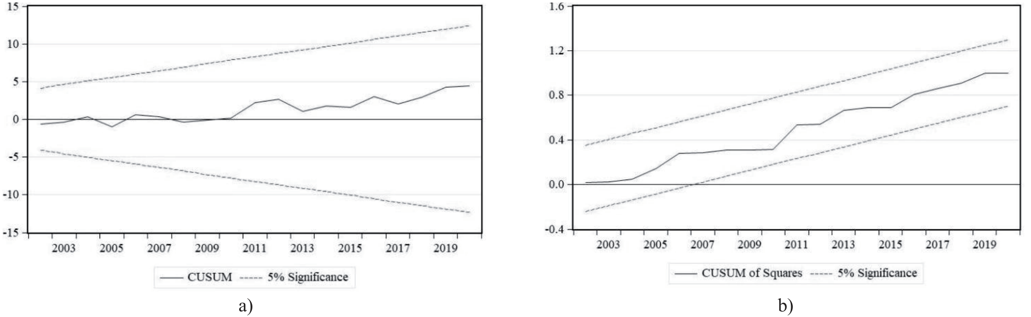
Fig. 2.
Stability test results for GHG emissions: a) Cumulative Sum (CUSUM) test and b) Cumulative Sum of Squares test.
To ensure the robustness of our ARDL estimations, we employed the fully modified ordinary least squares (FMOLS) model (see Table 4). Remarkably, the results obtained from FMOLS closely mirror those from the ARDL estimations. Specifically, we found that fossil fuel consumption and meat production exhibit positive and statistically significant effects on GHG emissions in Indonesia. Moreover, forest cover continues to demonstrate significant negative impacts on GHG emissions. Furthermore, we utilized the dynamic ordinary least squares (DOLS) method to further explore the long-run relationship among the variables (see Table 4). Interestingly, the results are quite similar to those obtained by the ARDL model. This consistency across different estimation techniques highlights the robustness of the observed relationships and enhances confidence in the validity of our results.
Error-Correction Model and Short-Run Determinants
This study also examined the short-run relationship between GHG emissions, fossil fuel consumption, meat production, and forest cover. The results obtained from the error-correction model are presented in Table 5. It was revealed that in the short-run, fossil fuel consumption and forest cover influence GHG emissions. In contrast, meat production was revealed to have no statistically significant impact on GHG emissions in the short-run. It was found that a 1% increase in fossil fuel consumption in the short-run is expected to bring about on average a 0.12% increase in GHG emissions in Indonesia. However, a 1% increase in forest cover is expected to bring about on average a 2.32% decrease in GHG emissions in the short-run, ceteris paribus. Notably, forest cover emerged as the most influential factor in reducing GHG emissions in the short-run, aligning with the perspective of [65] on the significant role of forests in mitigating atmospheric GHG levels such as carbon dioxide.
Another crucial finding highlighted in Table 5 pertains to the error-correction term (ECTt-1). This term measures the rate at which short-run disequilibrium adjusts towards long-run equilibrium [64]. The estimated coefficient of the ECTt-1 is negative and statistically significant at the 1% level of significance. This outcome provides additional evidence supporting the existence of a cointegration relationship among the variables, consistent with the results obtained from the ARDL Bounds testing procedure. Specifically, the coefficient of the ECTt-1 is -0.705, indicating that approximately 70.5% of the deviation from the long-term trajectory of GHG emissions in Indonesia is corrected annually.
Diagnostic Tests
The validation of the presented model was conducted through various diagnostic tests assessing stability and the hypotheses regarding the residuals, including no serial correlation, homoscedastic errors, model specification, and normality. The results of these diagnostic tests are summarized in Table 6. The probabilities associated with each test used to verify these hypotheses were found to be greater than the 5% level of significance. Consequently, the diagnostic tests confirmed the absence of serial correlation, homoscedastic errors, correct model specification, and normally distributed errors. Moreover, the stability of the coefficients was assessed through CUSUM and CUSUM of Squares plots. These plots demonstrated that the cumulative residuals and the squares of cumulative residuals remained within the bounds of the interval associated with a 95% confidence level (refer to Fig. 2). As a result, based on these comprehensive results, the model is deemed validated and capable of producing robust results.
Conclusion and Implications
This study investigated the relationship between fossil fuel, meat production, and forest cover on GHG emissions in Indonesia using annual data for the period 1990 to 2020. The time-series properties of the data were investigated using the ADF and PP unit root tests. Both unit root tests concluded that the variables were non-stationary in levels but stationary in the first difference. The bounds test approach to cointegration by [62] was used to explore the possible long-run equilibrium relationship among the variables. Having confirmed that the variables all shared a long-run equilibrium relationship, an error-correction model was estimated to obtain the short- and long-run relationship among the variables. It was found that in the long-run, fossil fuel use and meat production positively affected GHG emissions, while forest cover reduced atmospheric GHG. In contrast, in the short-run, fossil fuels had a positive relationship with GHG emissions, while forest cover had a negative relationship. Meat production was found to have no statistically significant impact on GHG emissions in the short-run. The error-correction term of 0.705 revealed that approximately 70.5% of the disequilibrium in the short-run is correct each year until long-run equilibrium is achieved. The ARDL model was evaluated using FMOLS and DOLS estimators, which yielded similar results. All diagnostic tests confirm that the estimated parameters are reliable.
To address the complex dynamics of fossil fuel consumption, meat production, forest cover, and greenhouse gas (GHG) emissions in Indonesia, policymakers should prioritize concrete actions. First, promoting renewable energy sources and transitioning away from fossil fuels is crucial for long-term emission reductions. Second, stringent measures to preserve and expand forest cover are necessary to mitigate GHG emissions. Enhanced monitoring and enforcement mechanisms are essential for short-term emission reductions. Additionally, investing in climate-resilient agriculture and promoting public awareness and education are vital for sustainable practices. International collaboration to access resources and expertise will accelerate Indonesia's transition to a low-carbon economy. Implementing these recommendations will not only mitigate GHG emissions but also ensure environmental sustainability and resilience for future generations.
While this study provides valuable insights into the relationship between fossil fuel consumption, meat production, forest cover, and greenhouse gas (GHG) emissions in Indonesia, it is not without limitations. One limitation is the focus on only three variables as determinants of GHG emissions. Future research could explore additional factors such as renewable energy adoption, per capita income, green finance, and green technology to provide a more comprehensive understanding of emissions dynamics. Moreover, this study utilized annual data, which may overlook intra-annual variations in emissions. Utilizing monthly data could offer deeper insights into seasonal fluctuations and inform more targeted policy interventions; however, such data is not available. By addressing these limitations, future researchers can build upon the findings of this study and contribute to a more nuanced understanding of GHG emissions dynamics in Indonesia.