

Introduction
A river basin is a complex system characterized by its integrity, regional interconnectivity, and the interactions between its various components [1]. As a typical public good that spans multiple administrative regions, the water resources within these basins present serious risks to human health and the environment when polluted due to their spatial spillover effects and negative externalities [2, 3]. Furthermore, in these regions, industrial activities and local government governance measures are closely intertwined, making the management of river basin water pollution a matter that encompasses the interests of multiple regions and stakeholders, thus creating a complex dynamic interaction [4]. Furthermore, the fragmentation of regional jurisdictions often leads to challenges such as “free-riding” and the “tragedy of the commons” [5-8]. Consequently, promoting inter-regional collaborative governance is widely regarded as a critical element of comprehensive watershed pollution control. However, differences in geographical location, industrial structure, and levels of economic development across cities result in variations in the costs and benefits of pollution control, generating conflicts of interest that hinder cooperation in water pollution management [9]. Therefore, balancing the costs and benefits among regions and stakeholders remains a significant challenge in the process of cross-regional collaborative water pollution governance.
Existing research primarily focuses on the governance interactions between upstream and downstream regions or between the mainstream and tributaries. For example, Yuan et al. [10] first compared the optimal emission levels of multiple pollutants in upstream and downstream regions under both noncooperative and cooperative game scenarios. Chen et al. [11] demonstrated that basin-wide collaborative governance can foster cooperation and resource sharing between upstream and downstream regions, optimize water pollution control, and promote the sustainable economic development of the basin. Song et al. [12] introduced a water quality credit market and developed a stochastic differential game model of upstream and downstream efforts, discussing the optimal feedback equilibrium of watershed environmental quality under three different scenarios. These studies demonstrate that the governance measures of upstream local governments affect both the pollution burden on downstream local governments and the overall water quality. However, such studies typically focus on the strategic interactions within a vertical governance structure, often overlooking the unique interactions that may exist between the local governments on both sides of the river during the governance process. Joint prevention and control on both sides of trans - provincial river basins is a key and difficult issue in water pollution management [13]. The two major challenges driving this governance complexity are “high costs and insufficient internal motivation” and “unclear pollution liability” [14, 15], both of which hinder the effectiveness of transfer payments and reward–punishment mechanisms while weakening external enforcement. Nevertheless, the existing literature provides limited insights into this issue. Therefore, enhancing governance efficiency requires addressing cross-bank cooperation and competition through institutional innovation, cross-regional collaboration, and interest-balancing mechanisms [16, 17].
Scholars have primarily used the evolutionary game model to research the water pollution management problems between government and enterprises. Yang et al. [18] utilizes an evolutionary game model to compare scenarios with and without pollution rights trading and employs stability analysis and sensitivity testing using phase diagram techniques. Wang et al. [19] developed an evolutionary game model involving local governments, enterprises, and the public to analyze the stable strategies for cooperative water pollution control in the Yangtze River Basin. However, due to information asymmetry and the limited rationality of the participants, it is difficult for stakeholders to achieve equilibrium through a one-time decision. In contrast, the differential game model allows for the dynamic representation of the continuous decision-making process of both the government and enterprises at different time points, better capturing the timeliness and policy flexibility inherent in real-world governance [20, 21]. More importantly, transboundary water pollution management involves not only local governments but also industrial enterprises and the central government. Industrial enterprises directly impact pollution levels through their emission reduction efforts [22], while the central government shapes policies, provides subsidies, and sets standards that guide and constrain the actions of local governments and enterprises [23]. However, existing research often overlooks the roles of enterprises and the central government, limiting a comprehensive understanding of the dynamics of water pollution governance.
Existing research on upstream and downstream water pollution and air pollution control provides important policy insights for addressing cross-border water pollution, especially in the context of climate change [24]. The former focuses on the stability of collaborative alliances [25] and the distribution of costs and benefits [26], while the latter examines the effectiveness of policies such as central regulation [27] and goal assessment [28] in regional pollution management. However, the applicability and implementation pathways of transferring these regulatory policies remain to be explored. The two main approaches to ecological compensation are fiscal transfers, where the government compensates affected regions [29, 30], and market-based mechanisms [31, 32], like carbon trading, which incentivize ecological preservation through market transactions. Liu et al. [33] showed that the Ecological Compensation Policy in river basins significantly optimizes industrial structures, while its impact on economic growth and technological advancement remains inconspicuous. Xu et al. [34] concluded that bilateral ecological compensation between upstream and downstream regions most effectively reduces pollutant emissions, making it the optimal form of ecological compensation. However, compared to the ecological compensation mechanism, the cost-sharing approach offers greater adaptability and flexibility. Yang et al. [35] developed a Stackelberg game model based on a cost-sharing mechanism for a Y-shaped river basin. Through numerical analysis, they demonstrated that this mechanism can enhance the effectiveness of pollution elimination, achieving Pareto improvements in both environmental and economic domains.
The main contributions of this paper are as follows. (1) We shift the focus from the traditional upstream–downstream governance model to the largely underexplored cross-bank governance relationship in transboundary river basins. (2) We extend the game-theoretic framework to incorporate not only local governments on both banks but also industrial enterprises and the central government – stakeholders that have often been overlooked in prior studies.
(3) The competition factor between local governments on both sides of the river is considered, capturing how economic development pressures lead to reduced pollution control efforts. (4) The differential game model is used to analyze the pollution control efforts of governments and enterprises from a dynamic perspective.
Materials and Methods
Establishment and Solution of Differential Game Models
Model Assumptions
Assumption 1: Consider a trans-jurisdictional river basin where the left and right banks (GL and GR, respectively) are governed by adjacent but independent local governments, each responsible for water pollution control within their jurisdictions. Meanwhile, the central government (GC) formulates macro-level governance policies for the entire river basin. Industrial production activities occur on both sides of the river, with industrial enterprises (E) discharging wastewater into the river, thereby acting as the primary sources of pollution.
Assumption 2: Industrial production activities on both the left and right banks discharge wastewater containing organic matter and various pollutants into the river. Let the total pollutant emissions from industrial enterprises on the left bank be denoted as qL, qL>0, and those from the right bank as qR, qR>0. The central government may impose an environmental protection tax ω>0 on local governments based on pollutant emissions, aiming to guide their pollution control decisions.
Assumption 3: Let the pollution control efforts of GL, GR, and GC be denoted as uL, uR and uC, respectively, where 0<uL, uR, uC<1, which reflects the policies, personnel, and financial investments of these governments. Additionally, the pollution control efforts of E are represented by uE, 0<uE<1, indicating efforts to reduce pollutant emissions through technological upgrades, end-of-pipe treatment, and clean production methods. Following the established literature (e.g., Gao et al. [36-38]), the cost of pollution control for each stakeholder is represented as a quadratic function of their respective effort levels. Therefore, the cost functions of each participant in the wastewater treatment process are represented as shown in Equation (1).
Where k>0 is a coefficient capturing cost discrepancies between the two regions and c>0, e>0 represent the cost coefficients for GC and E, respectively.
Assumption 4: E's utility function at time t can be represented as follows:
Where ψ>0 is the social reputation impact coefficient of wastewater treatment and δ(δ>0) is the external influence coefficient of water pollution control on the firm.
Assumption 5: The reduction of pollutants within the basin results from the collective efforts of GL and GR, GC and E, assuming that their unit pollution control efforts eliminate the following amounts of pollutants, respectively: ξ, η, θ and φ. Formally, the differential equation can be described as follows:
Where q(t) represents the effectiveness of pollution control, while α denotes the marginal diminishing efficiency of pollution treatment.
Assumption 6: Under economic development pressures, the two local governments on the river’s banks exhibit reluctance to independently undertake high-cost pollution control measures. To capture this effect, we define a competition coefficient β∈[0,1]. A higher value of β indicates a stronger tendency for both bank governments to reduce their pollution abatement efforts in response to economic constraints, reflecting heightened competitive pressures that favor development goals over environmental quality.
Without competition or central government supervision, the baseline pollution control efforts of GL and GR are uL0 and uR0. When competition and oversight are introduced, their efforts become:
Where β∈[0,1] captures the influence of economic pressures on reducing their efforts, and d1, d2>0 represent the central government’s regulatory impact on their actions. For the industrial enterprise, its abatement effort uE depends on local government pressure and policies, and is modeled as:
Similarly, d3>0 represent the extent to which the regulatory intensity of GL and GR influences the industrial enterprise’s behavior, indicating that stronger oversight and more stringent policies lead the enterprise to invest more in pollution reduction.
Assumption 7: Pollution control contributes to overall social welfare as captured by the relation:
Where S0 denotes the initial welfare level, and λ>0 represents the incremental coefficient reflecting how improvements in pollution abatement translate into higher social welfare.
Assumption 8: The conversion of changes in social welfare into respective benefits varies among GL, GR and E. Let πL, πR, πE>0 denote their distinct benefit conversion coefficients, reflecting differing economic development levels and regional conditions. Additionally, all stakeholders employ a common discount rate ρ>0, indicating a uniform temporal valuation of future payoffs across the central government, local governments, and the enterprise.
Non-Cost Sharing Scenario
In the Nash noncooperative game scenario, all parties make independent decisions.
The objective function of GL is JGLN:
Here, the parameters μi(i = 1, 2) represent the economic benefits each local government obtains from the other’s pollution-control efforts. χ represents the spillover effect coefficient of enterprise governance. And ri(i = 1, 2, 3, 4) respectively represent the governance marginal utility coefficients of GL, GR, GC and E.
The objective function of GR is JGRN:
The objective function of GC is JGCN:
The objective function of E is JEN:
Cost-Sharing Scenario
In this case, the central government funds pollution control and allocates cost-sharing ratios (m1, m2, 0<m1 + m2<1) to the left-bank and right-bank regional governments [39, 40], while the regional governments provide subsidies (n1, n2, 0<n1 + n2<1) to incentivize industrial enterprises’ pollution control efforts. At this point, the objective functions of each game participant can be expressed as Equations (11) to (14):
Results and Discussion
Non-Cost Sharing Scenario
To obtain the Markov Perfect Equilibrium solution for the non-cost sharing game, a set of bounded, continuous, and differentiable value functions
According to the first-order necessary conditions, the first-order partial derivatives of the right-hand side of Equations (15) to (18) with respect to uL, uR, uC and uE are set to zero. The equilibrium solutions of the game can then be derived as follows:
(19)
The expression for
By the substitution method, substituting Equation (21) into Equations (15)-(18) yields the following expressions:
(22)
By substituting Equation (21) into Equation (19), the optimal control strategies for each participant can be obtained as follows:
(25)
By substituting Equation (21) and (22) into Equation (20), the optimal payoff functions for each participant are obtained as follows:
At this point, the optimal value of social welfare is:
Cost-Sharing Scenario
In this game model, the central government shares a certain proportion of the pollution control costs with the left-bank and right-bank regional governments. The regional governments, in turn, provide incentive subsidies to the enterprises within their respective jurisdictions. The amount of subsidies provided by the regional governments is linked to the pollution control efforts of the enterprises. The objective functions of the participants can be expressed as:
(32)
(33)
(34)
The equilibrium solutions of the game in the cost-sharing mechanism can be obtained as Equations (36).
(36)
Similarly, the value function is a linear function of q(t). Thus, using the method of substitution of coefficients, the following equations are obtained:
Substituting Equation (37) into Equation (36), the following result is obtained:
(40)
Then, substituting Equations (38)-(41) into the central government’s HJB and setting the first-order partial derivatives of the right-hand side with respect to mi, ni(i = 1, 2) to zero, we obtain Equations (42):
(42)
By substituting Equation (38)-(41) into the objective functions of both the left-bank and right-bank local governments, and applying the first-order necessary conditions by setting the partial derivatives with respect to n1 and n2 to zero, the following results are obtained:
(43)
The optimal benefit functions for all participants are presented as shown in Equation (44) to (47):
(44)
(45)
(46)
Under the cost-sharing mechanism, the maximum social welfare is shown in Equation (48).
The following steps involve deriving and comparing the optimal control strategies of each participant under both scenarios.
According to Equations (23) and (38), we obtain:
(49)
Therefore, the cost-sharing mechanism not only increases the pollution control investment of industrial enterprises but also reduces the pollution control expenditure of local governments on both sides and the central government. Due to the complexity of the equilibrium solution, the impact of certain parameters cannot be directly determined. Therefore, it is necessary to conduct numerical analysis to identify the impact patterns of these parameters.
Numerical Simulation
In this section, the water pollution management model is simulated from the perspective of multiple stakeholders using MATLAB software, with exogenous variables assigned specific values. The parameter settings in this study are grounded in real-world scenarios and fundamental assumptions, with the values chosen based on these assumptions and informed by the relevant research, particularly the work of YANG et al. [41]. The initial assumptions for the model’s parameters are as follows: α = 0.01, β = 0.7, ω = 2, r1 = 0.06, r2 = 0.06, r3 = 0.06, r4 = 0.07, φ = 0.18, μ1 = 1, μ2 = 1.2, χ = 3, λ = 1.5, πL = 0.7, πR = 0.75, πE = 0.45, δ = 1.22, n1 = 0.2, n1 = 0.3, m1 = 0.2, m2 = 0.2, k = 2, c = 2, e = 2, ψ = 1.5, η = 0.15, θ = 0.13, ξ = 0.15.
As illustrated in Fig. 1 through Fig. 3, the implementation of the cost-sharing mechanism significantly improves wastewater treatment outcomes and enhances social welfare. Additionally, it leads to substantial increases in the profits of all participating stakeholders. This demonstrates that by distributing the financial burden among the involved parties, the mechanism not only boosts the overall efficiency of environmental management but also fosters the sustainability of the system.
Fig. 4 illustrates that as the competition coefficient increases, the local governments face heightened economic pressures, which may drive them to prioritize economic growth over environmental concerns. This results in a reduced focus on pollution control efforts, further exacerbating the overall decline in pollution management efficiency and profit (Fig. 5). Consequently, the negative impact of increased competition on environmental governance becomes more pronounced.
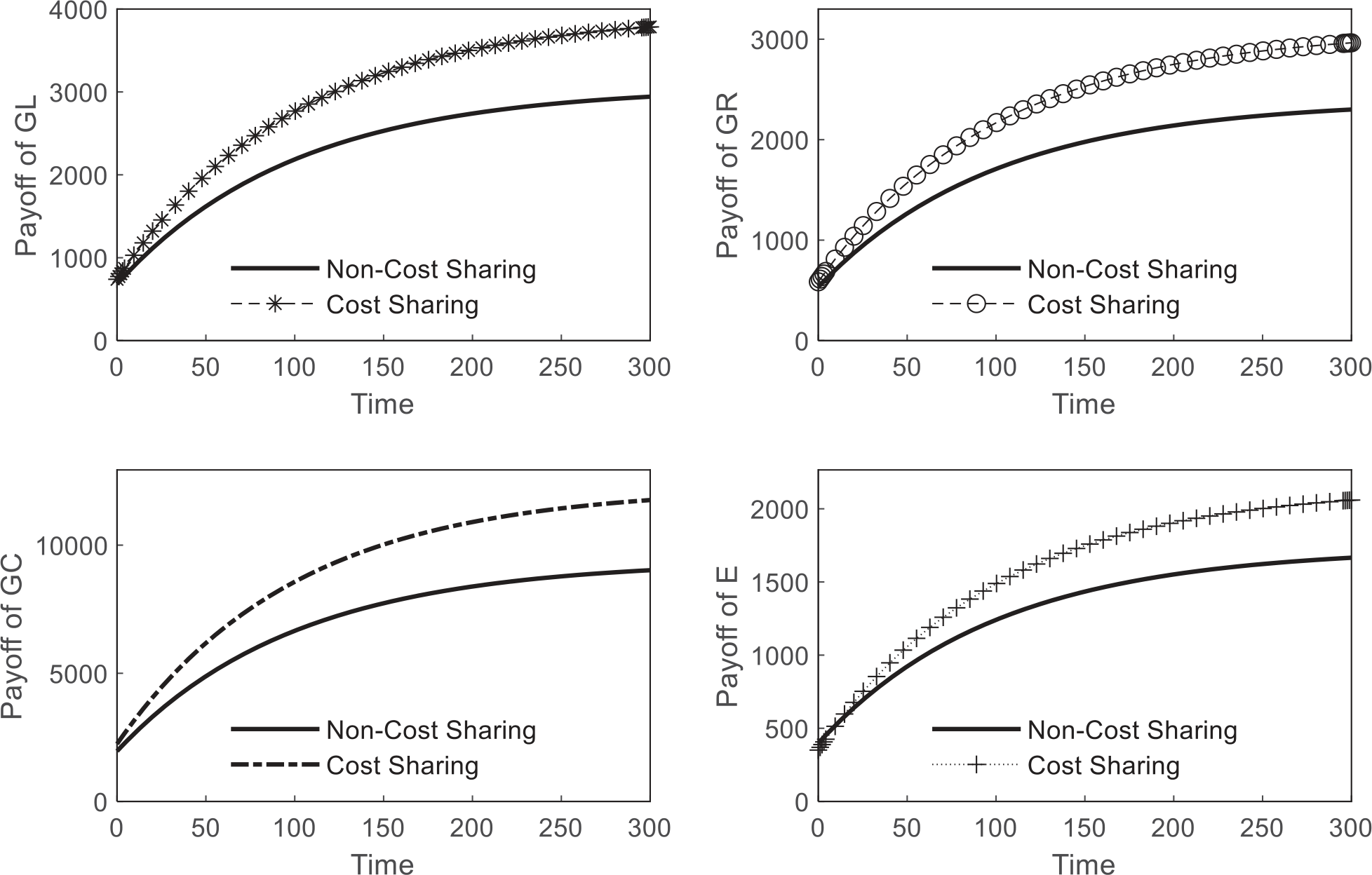
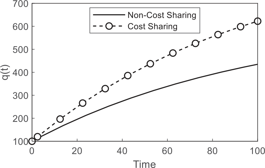
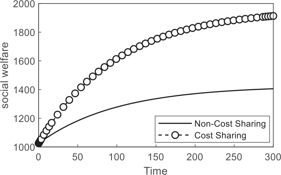
Fig. 4.
The impact of the economic competition coefficient between the two banks on the governments’ optimal effort.
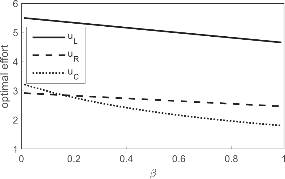
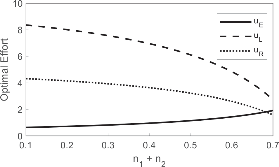
Fig. 6 illustrates that subsidy policies can significantly increase the pollution control efforts of industrial enterprises and help alleviate the financial pressure on the governments of both sides regarding wastewater treatment.
Fig. 7 indicates that the pollution control subsidy policy for enterprises effectively enhances the overall welfare. However, as the subsidy ratio increases beyond a certain threshold, the revenues of the local governments on both banks begin to decline. This suggests that determining the optimal subsidy coefficient is crucial to balancing the benefits of pollution control with the financial sustainability of government resources.
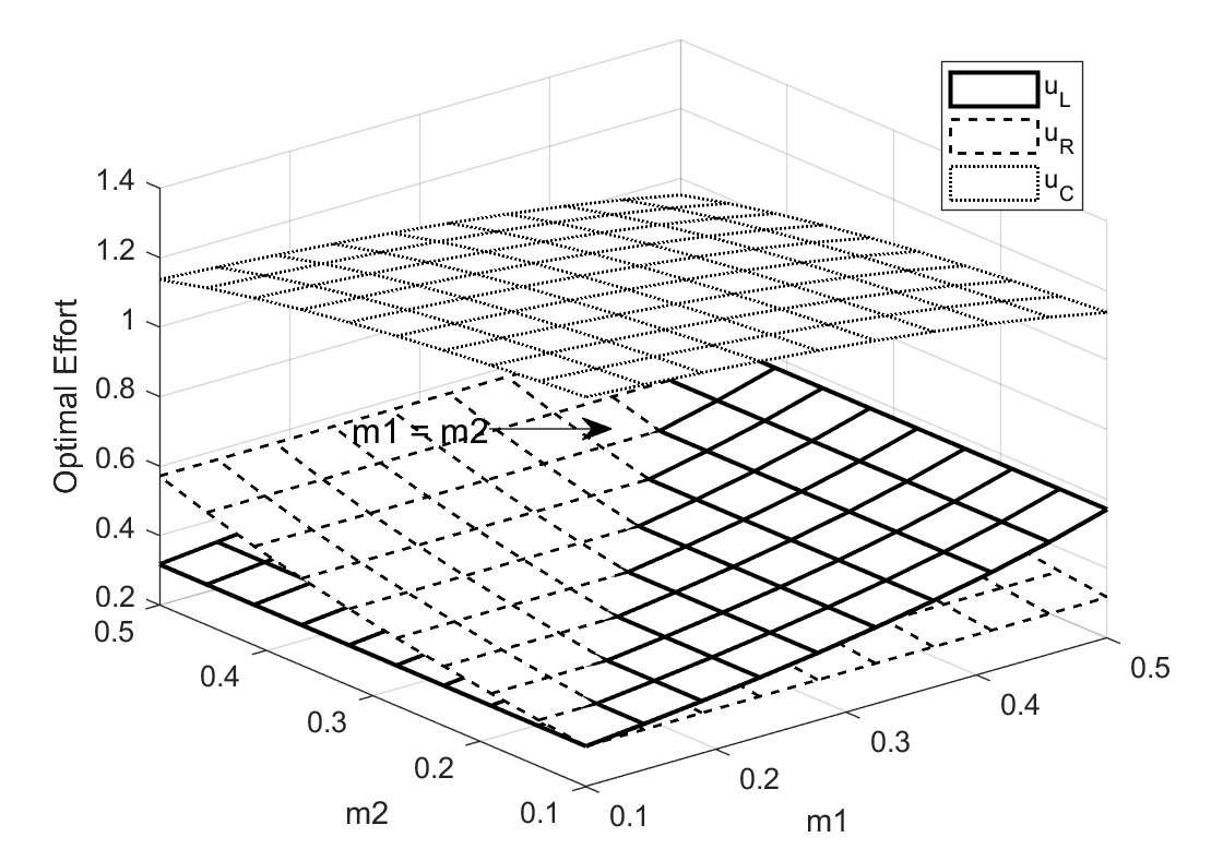
As shown in Fig. 8, an increase in the cost-sharing ratio effectively incentivizes local governments to increase their investments in pollution control. Moreover, this mechanism reduces the financial burden on the central government, allowing it to allocate more resources to other areas.
Conclusions and Suggestions
This study underscores that cost-sharing mechanisms between central and local governments significantly boost pollution control efforts, improve environmental quality, and enhance economic returns and social welfare. When the central government shares costs, local governments and enterprises face reduced financial burdens, promoting sustainability and more robust governance. By contrast, in the absence of cost-sharing, local governments under strong economic pressure often underinvest in pollution control as competition intensifies, ultimately undermining water quality and long-term benefits.
Fig. 5.
The impact of the economic competition coefficient between the two banks on the governments’ profit.
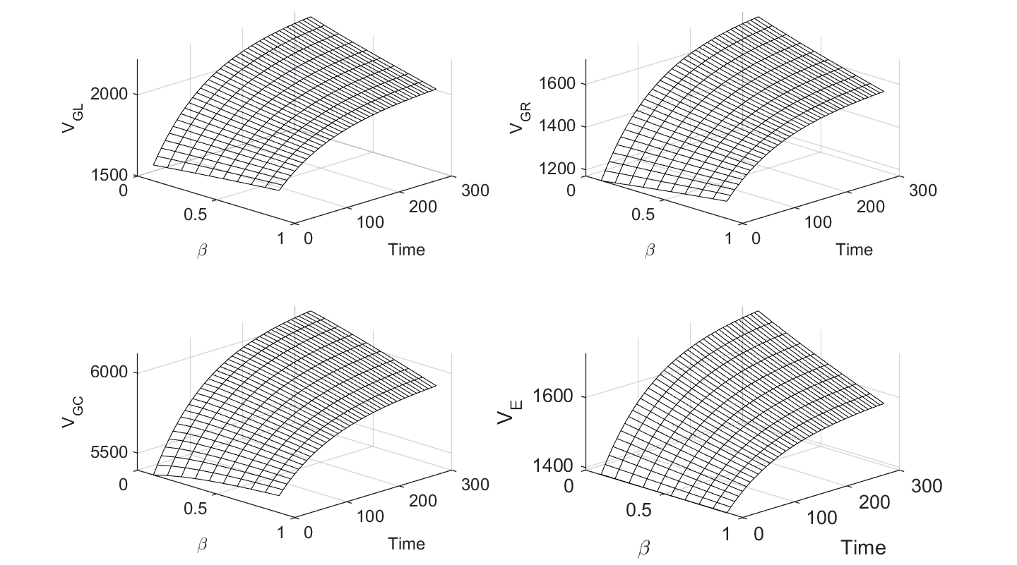
Fig. 7.
The impact of the sum of the subsidy coefficients for industrial enterprises by the two banks’ governments on the government’s optimal profit.
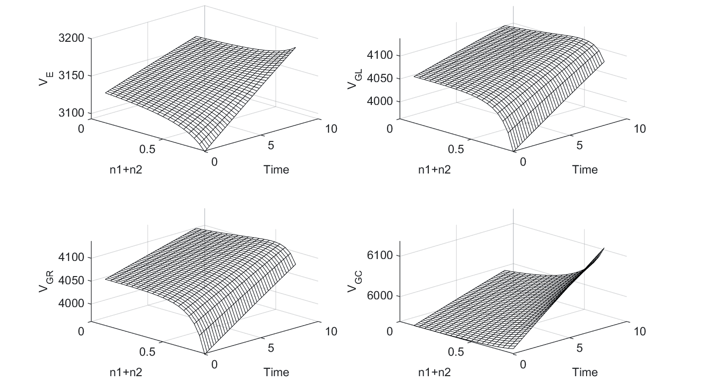
Fig. 8.
The impact of the central government’s cost-sharing coefficient (m) on the pollution control efforts of each participant by the governments on both banks.
To address these issues, the central government should strengthen oversight to ensure policy consistency across transboundary water bodies. In regions under considerable economic strain, targeted financial and technical support can further reinforce pollution management. Increasing the central government’s cost-sharing ratio and linking funding to pollution control performance can incentivize more effective local strategies. Local governments, for their part, can implement differentiated subsidies based on the pollution control capacities of industrial enterprises, thereby encouraging greater investment and fostering cross-regional collaboration. By sharing technologies and experiences, local governments can balance resource allocation and generate collective benefits. Additionally, implementing environmental tax policies and intensifying the assessment of corporate environmental performance can motivate enterprises to adopt responsible practices and invest more in pollution mitigation.
To further enhance pollution control efforts, it is recommended to introduce transparent monitoring tools, such as real-time water quality monitoring systems and IoT technologies, to improve pollution source tracking and management, thereby enhancing transparency and the effectiveness of governance. Additionally, exploring cutting-edge technologies, such as reverse osmosis membrane technology and AI-driven optimization of wastewater treatment processes, can increase the efficiency of pollution control, reduce energy consumption, and promote innovation in industrial wastewater treatment.
A limitation of this study is its reliance on hypothetical parameters due to limited real-world data, which may affect its generalizability. Moreover, the model does not fully capture the potential nonlinear factors in environmental and economic systems, which is our next research focus.

