

Introduction
According to the World Health Organization (WHO) assessment report, approximately 7 million individuals globally succumb to air pollution annually [1]. Consequently, air pollution has emerged as the paramount environmental health risk worldwide [2, 3]. As one of the major air pollutants, PM2.5 has been shown in numerous studies to pose undeniable hazards to human health [4-7]. Air quality monitoring data are the primary source for analyzing air pollution trends and modeling pollutant concentrations, holding immense significance for research in air pollution prevention and control. However, several factors—including the instability of automatic air quality monitoring systems, machine malfunctions, and human error—result in a substantial number of missing values in real-time air quality monitoring data [8]. This poses significant limitations on related air pollution research [9]. Therefore, the challenge of effectively imputing missing values in historical time-series data urgently needs to be addressed.
The current approaches for interpolating missing values are derived from data classification and regression prediction basic theory [10]. Based on the autocorrelation of data, Junger and Deleon used the Autoregressive Integrated Moving Average (ARIMA) model to estimate random missing values in time series, with experiments confirming that this method resulted in a satisfactory filling effect in univariate time series [11]. However, as missing data are often associated with multiple factors, some scholars [12, 13] used the K-Nearest Neighbors (KNN) algorithm to measure the degree of similarity between the data from the interconnections between the data values, thereby estimating the values of missing data through the same class of observations. KNN has a wide range of applications in real-world missing data imputation and has been applied to various fields with higher accuracy than regression interpolation [14-16]; however, the selection of value K (the number of neighboring labeled values) has a significant impact on the interpolation accuracy, so selecting the appropriate value for K is still a challenge [17]. Multiple Imputation (MI) generates a set of complete datasets through estimation and repeated simulation, filling the missing data in each dataset using the estimation model [18, 19]. However, this approach is sensitive to the models’ assumptions, and inappropriate assumptions may lead to bias [20]. Tashiro et al. [21] proposed the Conditional Score-based Diffusion Models for Imputation (CSDI) for missing values imputation of time series data, demonstrating that CSDI could fill the missing data by utilizing the observed valid information. However, CSDI has not been used to fill in missing air quality monitoring data. The variables of air quality monitoring data are not only spatiotemporally correlated but also interdependent with other variables. Therefore, it is necessary to deeply analyze the missing data characteristics of air quality monitoring data and explore the filling effect under different scenarios.
Based on an in-depth analysis of the characteristics of missing data values in actual sample data, this study designed experiments from the perspectives of missing data rates and missing data scenarios. Then, multiple algorithms were compared, and the missing data from air quality monitoring sites in the Yangtze River Delta (YRD) were interpolated and analyzed based on K-Shape to complete the air quality monitoring datasets.
Materials and Methods
Study Area
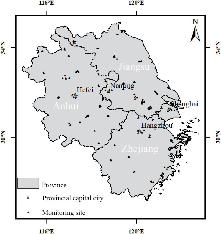
The YRD region is in the lower reaches of the Yangtze River in China, between latitude 26°58’N and 35°10’N and longitude 114°54’E and 122°50’E. It consists of 41 cities in the Shanghai Municipality, Jiangsu, Zhejiang, and Anhui Provinces and covers an area of 358,000 km2. Spanning north and south, the YRD presents great variations in topography and geomorphology, with plains in its north, mostly mountainous and hilly areas in its southwest, and cities in its east adjacent to the Yellow Sea and the East China Sea (Fig. 1). The YRD has a predominantly subtropical monsoon climate, characterized by high temperatures and rainy summers and cold, dry winters [22]. The YRD is densely populated and is one of China’s most seriously air-polluted regions [23, 24]. It is also one of the key regions in China that promotes the joint prevention and control of air pollution [25]. There are 235 air quality monitoring sites and 69 national meteorological monitoring sites in the YRD, with most of the air quality monitoring sites located in urban areas and meteorological monitoring sites sporadically distributed in most cities.
Data
This study collated PM2.5 hourly concentrations from 235 monitoring sites in the YRD during 2015- 2020 via the China Environmental Monitoring General Station (http://www.cnemc.cn/). The monitoring process of PM2.5 concentrations is strictly in accordance with the ‘Technical Specification for Operation and Quality Control of Continuous Ambient Particulate Matter Automatic Monitoring System’ (HJ817-2018). Each PM2.5 hourly concentration value is the arithmetic average of the data output from the instrument every five minutes during an hour, and all valid data have gone through a series of audit steps to ensure their accuracy and validity. After cleaning and sorting the data from the 235 monitoring sites, 172 valid sites were retained, excluding those with a missing rate of more than 20% and those that did not include all the years in the study period.
Methods
Imputation Methods
(1) The ARIMA model is a differential autoregressive moving average model combining the autoregressive model (AR), moving average model (MA), and difference method. It is denoted as ARIMA (p, d, and q), where p is the self-regulating order, d is the differential number, and q is the mobile average number. It is one of the most common methods for time series analysis in practical applications [26-29]. The advantages of the ARIMA model are its simplicity and ease of use, as it only requires the autoregressive variables to forecast rather than other covariates; its disadvantage is that it requires the time series data to be stable after differentiation and cannot capture the nonlinear relation [11, 30]. The basic steps of the ARIMA model are as follows:
(a) Observe whether the time series is stationary by plotting. For a non-stationary time series, perform d-order differencing to transform it into a stationary series.
(b) For the stationary time series obtained in step (a), calculate its autocorrelation coefficient (ACF) and partial autocorrelation coefficient (PACF). Analyze the autocorrelation and partial autocorrelation plots to determine the optimal order of the autoregressive term p and the moving average term q.
(c) Based on the p, d, and q values determined in the previous steps, conduct model diagnostics for the ARIMA (p, d, and q) model to select the best model for data forecasting.
This study used the Forecast package in the R programming language to determine the ARIMA deficiency value and automatically select the p, d, and q values using the Auto.arima function. Auto.arima was selected to automatically determine (p, d, and q) parameters due to its robustness in optimizing Akaike Information Criterion (AIC) and Bayesian Information Criterion (BIC) metrics, as validated by Hyndman and Khandakar [31]. In this study, the number of monitoring sites was large, so the automatic tuning of parameters using Auto.arima also had significant scalability compared with manual tuning [32].
(2) MI is a method for dealing with missing values based on repeated simulations. Basically, a set of complete datasets is generated from a dataset containing missing values, and then the same method is used to process each complete dataset. Finally, the processing results are synthesized to obtain an estimate of the target variable [33]. This study used the MICE package in the R programming language to perform MI. First, the Fully Conditional Specification (FCS) method in the MICE function generated five interpolated datasets based on Rubin’s rules [34] and empirical evidence [35]. Then, the “with” function applied a linear model to the interpolated five complete datasets for statistical analysis. Finally, the “pool” function integrates the five separate analysis results into a group result.
(3) The core of the KNN algorithm is that if most of the K nearest samples of a sample in a feature space belong to a certain category, then the sample also belongs to this category and has the characteristics of samples in this category [36]. KNN can be used to interpolate the missing samples simply and effectively, but approaches for determining the optimal adjacent value K are still the focus of debate. In this study, the KNN imputation function in the DMWR package in the R programming language was used to fill in the KNN deficiency value. The K value cycled from 3 to 20 to select the value with the minimum error rate for the test set.
(4) CSDI is a probabilistic interpolation diffusion model based on conditional scores, which connotes the interpolation of known values as conditional information using a score-based diffusion model. The model interpolation training process is as follows:
(a) Noise data equal to the length of the original data sequence is prepared, and the valid values of the original dataset are divided into two parts: the target
(b) The missing part of the dataset is filled into a complete sequence
(c) The noise data is added to the filled target, and the target data containing noise is denoted as
(d) The time information, observation data, target data, and mask information are input into the denoising diffusion probability model (DDPM). The observed conditional information is used to simulate the true distribution of the data to remove the noise in the dataset to be interpolated. Parameterization of the denoising function is shown in Equation (1):
Here, μDDPM and σDDPM are untrainable functions, εθ is a trainable denoising function that estimates the noise added to the original data given the noise data and the observation data, and t = 1,2...,T is a hidden time series. For details, please refer to the original CSDI paper [21].
(e) Iterative training is performed to obtain the optimal estimate of the model simulation. The loss function for model training is shown in Equations (2) and (3):
Here, x0 is the original data without noise, q(x0) is the distribution of x0, ε is the noise sampled from the standard normal distribution N(0,I), m is the observation mask information of the data, {a1:T} is a noise level sequence that satisfies 1>a1>...>aT>0, and
This study selected the original dataset of the PM2.5 concentration ground monitoring sites from 2016 to 2017 for modeling. Data from February, May, August, and November were taken as observation objects; data from January, April, July, and October were taken as target objects; and data from March, June, September, and December were taken as test data. To avoid multiple estimates for each missing value, 48 consecutive time steps were set as one window, and each month had no overlap of test data. When the length of one month’s data was not divisible by 48, the last sequence overlapped with the previous sequence, but the overlapped results were not aggregated. During each training iteration, data from one month were selected as validation data, and the remaining data were used as training data. The batch size was set to 16 for the hyperparameter settings to balance computational efficiency and training stability [37]. The model was trained for 200 epochs to ensure thorough convergence and effective pattern extraction [38, 39]. We adopted the Adam optimizer with an initial learning rate of 0.001 [40]. A scheduled decay was implemented: the learning rate was reduced to 0.0001 at 75% of the total epochs and further to 0.00001 at 90% of the total epochs, facilitating rapid convergence in the early training stages and fine-grained parameter optimization in the later phases [41, 42]. Following the channel configuration of DiffWave [43] and based on the validation loss and parameter size, the number of residual layers was determined to be four, with each residual layer having 64 channels.
K-shape
K-shape is a domain-independent, high-precision, and efficient time series clustering method with a wide range of applications proposed by Paparrizos and Gravano [44] for the clustering of time series data problems. In this study, the K-Shape algorithm was used to classify the similarity of 172 effective air quality sites in the YRD region, enabling exploration of the zoning based on the clustering results. The basic process of the K-shape algorithm is as follows:
(1) The distance between the two time series is calculated using the distance scale shape-based distance (SBD) measured by the correlation-based method.
(2) The center of mass is calculated according to the distance algorithm in step (1) so that it has the maximum similarity with each sequence in the cluster.
(3) The center of mass is recalculated based on the distance scale and center of mass formulae in steps (1) and (2). Different clusters are reassigned based on the distance of each sequence from the new center of mass, with iterative looping until the labels no longer change.
The most important aspect of using a clustering model is determining the number of cluster centers, that is, the number of clusters to be classified [45]. In this study, the elbow method and contour coefficients were used to determine the classification effectiveness of the K-Shape algorithm on the PM2.5 concentration time series. The basic principle of the elbow method is that an inflection point (i.e., the ‘elbow’ point) occurs in the process of iteratively calculating the change of the sum of squared errors (SSE) of the points and cluster centers under different numbers of clusters; this ‘elbow’ point is considered to be the optimal number of clusters. The contour coefficient combines the two factors of cohesion and separation of clustering, with the greater the similarity between samples within clusters and the smaller the similarity between samples between clusters, the better the clustering effect. The calculation of the contour coefficient S is shown in Equation (4):
Here, a is the average value of the degree of dissimilarity from point i to other points in the same cluster, b is the minimum value of the average degree of dissimilarity from point i to other clusters, and the value of S is in the range of [–1, 1]. The closer S is to 1, the better the clustering effect.
Evaluation Index
The root mean square error (RMSE), mean absolute error (MAE), and continuous ranked probability score (CRPS) were selected to measure the model’s performance. RMSE and MAE were used to measure the deviation between the predicted and true values and to reflect the distribution of the predicted values error, respectively. The CRPS was used specifically to evaluate the accuracy of CSDI. RMSE and MAE were calculated using Equations (5) and (6) [46].
Here yi is the measured value, fi is the model estimate, and
The compatibility of the estimated probability distribution F with the observations x using the CRPS metric can be defined as the integral of the loss function at the quantile level, as shown in Equation (7) [21]:
Assuming that the number of features and the number of time steps of the input data are K and L, respectively, the normalized average CRPS overall features and time steps is denoted as shown in Equation (8):
In this study, the probabilistic predictive evaluation of CSDI used the sum of CRPS of K features in the probability distribution F to compare the model performance. That is, the CRPS-sum is denoted as shown in Equation (9):
Missing Sample Construction
Taking the PM2.5 concentration samples from 2016 to 2017 as an example, the overall missing rate of 17,544 pieces of data was 4%. The types of missing sample data included missing data at random single sites for a given period (case 1) and missing data at multiple sites simultaneously for a given period (case 2). According to the distribution of missing values of samples, the missing rate of PM2.5 concentration ground monitoring data was far below 20%, and the missing periods of monitoring sites were not completely uniform. Therefore, based on the analysis of potential correlation and autocorrelation between sites and other sites, the missing time series of PM2.5 concentration could be effectively filled. According to a case 1:case 2 ratio of 1:4, a mixed dataset with missing ratios of 5%, 10%, 20%, 30%, and 50% was constructed (i.e., 1%, 6%, 16%, 26%, and 46% virtual missing data were added based on a missing dataset of real samples).
Results and Discussion
Comparison of Imputation Methods
The comparison results of the four missing value imputation methods under different missing rates (Table 1) revealed that ARIMA had the poorest prediction accuracy. CSDI had the highest prediction accuracy, with significantly lower MAE and RMSE values than the other methods. When the missing rate was greater than 20%, the errors of the four methods significantly increased, with the ARIMA prediction error increasing the most. The prediction accuracy of CSDI did not change much when the missing rate was increased further, and the error at a 30% missing rate was almost the same as that at the 50% missing rate, corresponding to RMSE values of 9.35 and 9.4 µg·m–3, respectively. In general, CSDI was competent at filling the missing values of the PM2.5 monitoring data, and its prediction accuracy was less affected by the missing rate, while the prediction effect of the other three methods was greatly reduced when the data missing rate was greater than 20%. Therefore, CSDI has a significant advantage under high missing rate conditions, where conventional methods suffer from insufficient reference information, while the probabilistic framework of CSDI provides robust uncertainty quantification to maintain stable performance [21, 47].
Table 1.
Cross-validation results of the four methods under different missing rates.
Additionally, imputation experiments were also conducted using two well-known traditional methods, linear regression (LR) and polynomial regression (PR). It was found that CSDI also outperformed these traditional methods (Table 1). LR and PR inherently assume fixed functional relationships between variables (e.g., PM2.5 concentrations and meteorological factors), which oversimplifies the complex nonlinear interactions observed in real atmospheric systems [48-50].
A comparison of the filling effects of the four methods for two missing scenarios (Fig. 2) showed that both the ARIMA model and CSDI could effectively fill discontinuous missing data. In contrast, both the KNN and MI methods performed poorly in filling discontinuous missing data, and the imputation results were unstable (see Fig. 2a)); this may have been related to the insufficient learning ability of these models. The CSDI method still performed well in filling in continuous missing data and was markedly superior to the other methods. KNN and MI could enable the approximate estimation of continuous missing values, and the difference between the two methods was not significant. As an autoregressive method, ARIMA was inadequate in solving the problem of continuous missing data (Fig. 2b)). The comparison of the four methods across missing scenarios demonstrated CSDI’s considerable advantage compared to conventional methods in handling long-term continuous missing values. This superiority arises from CSDI’s conditional score-based diffusion mechanism, which effectively captures the evolving temporal correlations in non-stationary scenarios [51], a capability that conventional methods lack.
Missing PM2.5 Monitoring Data Imputation Using CSDI Based on Clustering Partitioning
Because of the spatial heterogeneity of air quality, it is necessary to analyze the time series and partition the air quality monitoring sites. The K-shape method was used to perform temporal cluster analysis on 172 effective sites in the YRD. When the number of cluster categories was set to four, elbow points appeared (as shown in Fig. 3), the elbow coefficient descending gradient was the largest, and the number of clusters was optimal. Accordingly, the sites were classified into Partition I (53 sites), Partition II (31 sites), Partition III (70 sites), and Partition IV (18 sites). As can be seen from the contour coefficient diagram in Fig. 3, the overall average contour coefficient tended to be 0.34, the average contour coefficient in Partitions I and II was small, and the classification effect was poor. Less than half of the sites had a contour coefficient greater than average. The average contour coefficient of Partition IV was the largest, and, except for two misclassified sites, the contour coefficient was greater than 0.34. The contour coefficient of the vast majority of sites in Partition III was higher than the average.
The results of the K-shape cluster analysis (Fig. 4) showed that the monitoring sites in Partition I were clustered in the central and western parts of the YRD and spread throughout Anhui Province. The average annual PM2.5 concentration from 2015 to 2020 was 47.87 μg·m–3, and this period had the most pronounced annual decline trend, with an average annual PM2.5 concentration in 2020 of only 35.33 μg·m–3. The monitoring sites in Partition II were clustered in the northern part of the YRD, in the northern cities of Anhui and Jiangsu provinces. The average PM2.5 concentration was the highest; the average PM2.5 concentration from 2015 to 2020 was as high as 55.72 μg·m–3, and the inter-annual decline trend was small. The monitoring sites in Partition III were clustered in the eastern part of the YRD, in Shanghai and some cities in Jiangsu and Zhejiang provinces. The average annual PM2.5 concentration from 2015 to 2020 was 42.26 μg·m–3, with a pronounced annual decline trend. The monitoring sites in Partition IV were clustered southwest of the YRD, mainly in Zhejiang Province. These had the lowest average PM2.5 concentration from 2015 to 2020 of 32.51 μg·m–3.
Fig. 2.
Imputation results of the four methods for a) univariate discontinuous missing data and b) univariate continuous missing data.
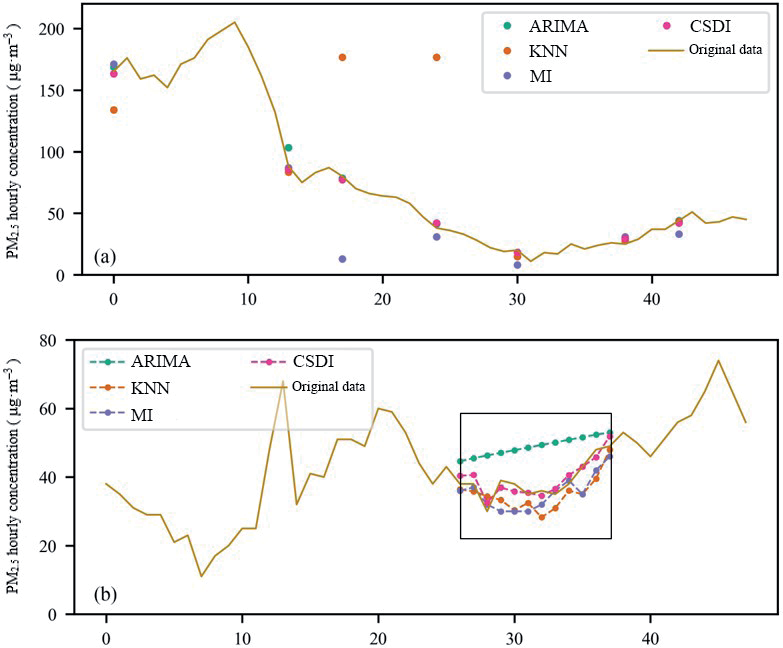
Table 2.
Prediction accuracy evaluation of CSDI in different partitions.
| Ⅰ | Ⅱ | Ⅲ | Ⅳ | Entire region | |
|---|---|---|---|---|---|
| RMSE | 7.83 | 8.55 | 5.4 | 5.78 | 10.69 |
| MAE | 5.17 | 5.3 | 3.26 | 3.27 | 6.72 |
| CPRS | 0.075 | 0.063 | 0.055 | 0.067 | 0.103 |
To improve the accuracy of the complete PM2.5 concentration dataset after filling, a PM2.5 sample set was constructed with a 20% missing rate (2016-2017) and divided into training sample sets by spatial partitioning. The results (Table 2) showed that the RMSE, MAE, and CRPS values of the entire region were 10.69 μg·m–3, 6.72 μg·m–3, and 0.103, with all indicators inferior to the filling accuracy of any partition. Therefore, capturing temporal and spatial correlation information based on spatial partitioning effectively improved the accuracy of the time series data prediction model.
Comparing the error evaluation of each partition revealed that the model error of Partition II was the highest, with an RMSE of 8.55 μg·m–3, and the model error of Partition III was the lowest, with an RMSE of only 5.4 μg·m–3. From the perspective of probability prediction, the predicted values distribution of the Partition III simulation was closer to the real values distribution. Although the RMSE and MAE values of Partition II were much higher than those of Partition IV, the probability prediction effect of Partition II was slightly better than that of Partition IV. The probability prediction effect of Partition I is the worst. This phenomenon was attributed to the poor classification effect of cluster analysis in Partitions Ⅰ and Ⅱ, as well as the different data distribution characteristics. This meant that CSDI tended to be smoother than the real dataset when interpolating missing values.
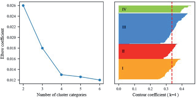
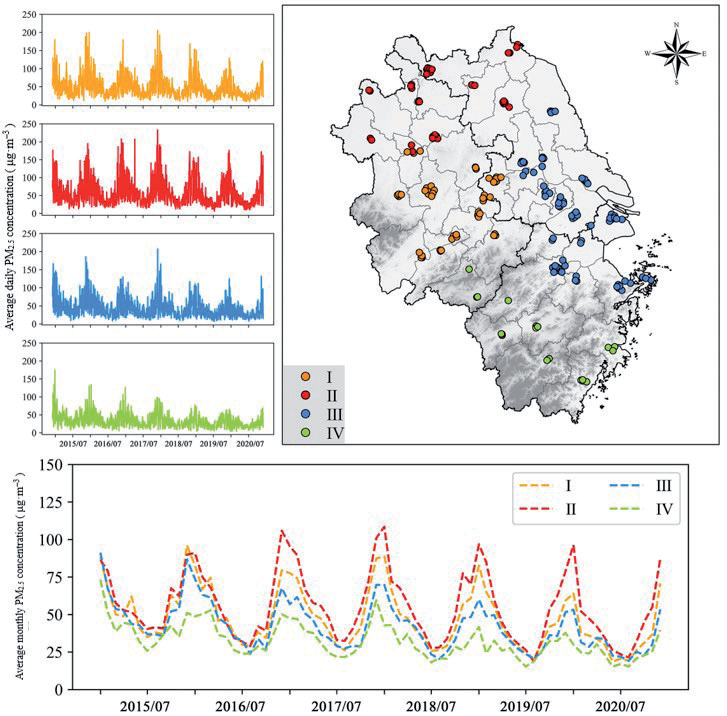
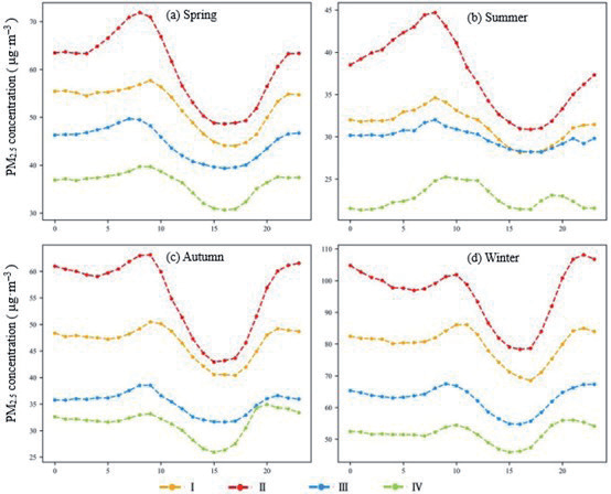
Fig. 5.
Daily variation trend in PM2.5 concentration in different cluster partitions in spring, summer, autumn, and winter.
It is noteworthy that while the K-shape clustering effectively captured temporal patterns in the YRD, the framework’s adaptability to regions with contrasting geographical and climatic conditions (e.g., plateau, coastal, or industrial zones) requires further validation. Studies have demonstrated that terrain-driven airflow stagnation [52] and monsoon-induced pollutant dispersion [53] can fundamentally alter PM2.5 diurnal cycles. Additionally, regional disparities in dominant emission sources—such as biomass burning versus vehicular emissions [54]—may challenge the assumption of intra-cluster homogeneity. Future implementations should incorporate geospatial covariates (e.g., elevation gradients, land-use types) into the clustering phase to enhance model generalizability across heterogeneous regions.
Daily Variation Characteristics of PM2.5 Concentrations in Different Spatial Partitions
To explore the important time nodes of the missing data imputation, this study analyzed the variation trend in the average hourly PM2.5 concentration in different cluster partitions in the four seasons from 2015 to 2020. The results (Fig. 5) showed that the daily variation in PM2.5 concentration in the four seasons in the YRD presented a fluctuating trend of increasing, then decreasing, and then increasing, with obvious ‘peaks’ and ‘valleys’. In the four seasons, the daily PM2.5 concentration variation curve presented a ‘peak’ and a ‘valley’ in the daytime and at night, respectively. The peak values in the daytime and at night were essentially the same in autumn. However, the peak PM2.5 concentration during the daytime in spring and summer was significantly higher than at night, while the reverse was true in winter. As follows, the specific periods and fluctuations of peak and valley values in different partitions were different in different seasons. In spring, the highest PM2.5 concentrations in Partitions II and IV were at 8 am, and in Partitions I and III, they were at 9 am and 7 am, respectively. The lowest PM2.5 concentrations in the four partitions were concentrated at about 5 pm, and the change in PM2.5 concentration tended to be flat from 2 pm to 6 pm. In summer, the highest and lowest PM2.5 concentration values in Partitions I, II, and III were at 8 am and 5 pm. In contrast to other partitions, Partition IV showed an ‘M’ pattern in summer, with the peak PM2.5 concentrations at 9 am and 7 pm. In autumn, the trend in PM2.5 concentrations in Partitions I and III was the same, with the highest values at 9 am and 9 pm. The highest values in Partition II were at 9 am and 11 pm, and the peak value at 8 pm in Partition IV was higher than at 9 am. The lowest values in each partition were at about 4 pm. In winter, the peak values of each partition at night were higher than the peak values in the day. The timing of the peak and valley values of Partitions I and II were the same, with the highest values at 10 am and 10 pm, respectively, and the lowest values at 5 pm. The PM2.5 concentration trend for Partitions Ⅲ and Ⅳ was similar, with the valley values at 3 pm and the peak values at 10 pm and 8 pm, respectively.
In general, the daily change in PM2.5 concentration had two peaks at approximately 9 am and 9 pm, as well as a valley at approximately 3 pm. The increases and decreases in different partitions in different seasons were slightly different, and the peak PM2.5 concentration at night in Partition IV appeared earlier than in other partitions. In terms of the fluctuation trend, the variation in PM2.5 concentration in Partition III was gentler than that of other partitions, and the variation fluctuation in Partition II was the largest; this was the main reason for the higher CSDI interpolation accuracy in Partition III and lowest interpolation accuracy in Partition II.
Conclusions
The main conclusions of this study were as follows.
(1) A comparison of the filling effects of the four missing value imputation methods under different missing rates and different missing scenarios revealed the CSDI to have the highest accuracy and the best filling effect overall.
(2) Based on the results of K-shape clustering partitioning, CSDI was used to fill the historical PM2.5 monitoring data of the YRD sites. The spatial partitioning effectively improved the CSDI’s filling effect. The filling error of the historical PM2.5 concentration data of the sites in Partition III was the smallest, and the filling error of Partition II was the largest; this was related to the site’s clustering accuracy as well as the characteristics of the data of different partitions.
(3) Analysis of the daily variation trend in PM2.5 concentrations in different seasons revealed that approximately 9 am, 3 pm, and 9 pm were the three main time nodes with large CDSI filling errors in the YRD region.
This study verified the effectiveness of CSDI in imputing real air quality monitoring datasets, demonstrating its significant practical relevance for air quality prediction. In practical applications, the trained CSDI can be integrated into air quality prediction systems, enabling it to receive new observational data in real time and perform imputation. Using the complete dataset obtained after imputation, it is possible to characterize the evolution of air pollutants more reliably and improve the accuracy of air quality prediction.
However, this study had some limitations, such as the lower interpolation effect of CSDI in the period of large PM2.5 concentration fluctuations. Improvements can be achieved via two approaches. First, develop a variant of the diffusion model based on Gated Recurrent Units (GRUs) and implement dynamic updates of model parameters through a sliding window mechanism (e.g., a 6-hour window). Trigger a real-time gradient update mechanism when the hourly change in PM2.5 concentration exceeds a set threshold. Second, Variational Autoencoders (VAEs) separate the fluctuation features driven by meteorology and those driven by anthropogenic emissions. Use the decoupled features as the conditional input for the diffusion model.

