

Introduction
Sustainable development (SD) is the common pursuit of all countries worldwide. The harmonious development of the relationship between humans and land is one of the important elements of SD. One of the typical manifestations is to coordinate the relationship between human production, life and environmental protection. However, rough production and lifestyle make the ecological environment deteriorate continuously. Air pollution [1], extreme climate [2], soil pollution [3], water pollution [4] and other environmental pollution problems continue to emerge. This makes the green development of living space and production space (PS) particularly important. The PS is related to the production function of land and production land. The production function is the ability of the land use system to provide a variety of products and services for human beings, which mainly depends on the natural output of the land and the results produced by human labor [5-7]. It is constrained by natural resources, the environment, and other regional indigenous factors [8]. The production land is related to industrial structure [9], and it mainly meets the needs of economic development [7]. It is used in agriculture, industry, business activities, and is used to get the product and provide the function of the land [10, 11]. Thus, PS refers to the agriculture, industry, and business for products and supply function space [12]. It is divided into agricultural production space and industrial production space [10, 13-15]. Exploring the ecological level of production space (ELPS) is to analyze the economic and ecological benefits brought by human production activities in the PS. This helps to find the problems existing in the process of SD in the PS. In China, the Yangtze River Economic Belt (YREB) has a strategic positioning of ecological priority and green development. The upper reaches of the Yangtze River (URYR) is the largest part of the YREB in China. It has 48% of the total water resources of the YREB. It is rich in natural resources and is a key zone for maintaining the ecological balance of the Yangtze River basin. Exploring the temporal and spatial evolution characteristics of ELPS in the URYR can not only provide a perspective for cities in the URYR to examine their own green development level, but also provide a reference for other ecological protection areas. At the same time, it is of great significance to promote the green development of the YREB.
It is tough to identify the PS of each city and then measure the quality level. Since the functions of production space, living space and ecological space (PLE) are often intertwined, overlapping, they form a single or composite function type [10]. Some scholars believe that the PLE are determined by the dominant function type [10, 15]. Other scholars believe that based on the multifunctionality principle, PLE are classified into many categories, like ecological space, living–productive space, ecological-productive space, and productive– ecological space [16] or living space, ecological space, industrial-production space, and ecological-production space [12]. Therefore, based on the macro- city spatial scale, this paper regards each city as a point like concentrated PS, and the healthy development of urban production space(UPS) is critical to the SD of the entire country. Therefore, the research object of this paper is UPS. The goal of this paper is exploring the temporal and spatial evolution characteristics of the ecological level of urban production space (ELUPS) in the URYR, and, ultimately, promote the green development of the URYR, even YREB.
At the present, there are abundant studies related to PS or ecologicalization, such as the identification of PLE [15], grain production space reconstruction [17], production space overheating forecast [18], ecological economics theory and model [19-21], ecological engineering [22], enterprise eco- development [23], industry ecologicalization [24, 25] or green development [26], infrastructure and green cities [27-29], urban development and regional green development [30, 31], urban green space [32-35], urban green development [36-38]. Among them, the urban green development is more closely related to the ecologicalization of production space (EPS) or ELPS, such as urban green development level [39, 40], urban green development performance [41], influencing factors of urban green development [42-44], urban green development transformation [45]. However, the focus is on the city as a singular entity, and the indicators do not fully account for the influence of its size. On the other hand, research into the EPS requires an examination of both economic and environmental benefits. Consequently, it is crucial to examine the input-output status of a space unit. This paper attempts to construct some input-output indicators of PS in terms of units of urban construction land, which are an integral aspect of the EPS indicator system. In addition, to our knowledge, there has been limited research conducted on the EPS, and even fewer empirical studies. Thus, this study can contribute to filling the gap in current literature.
Materials and Methods
The Study Area
From the perspective of natural conditions and economic connectivity, the URYR on a large scale mainly refer to Chongqing Municipality, Sichuan Province, Yunnan Province and Guizhou Province. It lies between 21°8′-34°19′N latitude and 97°21′-110°11′E longitude. The climate is dominated by subtropical monsoon climate. The land area is about 1,138,700 square kilometers. The elevation varies greatly, with the lowest point at 73.1 meters and the highest at 6740 meters. The landform is complex, mainly in mountains, hills, plains and plateaus. Its main tributaries are the Jinsha River, Yalong River, Jialing River and Wujiang River, etc.
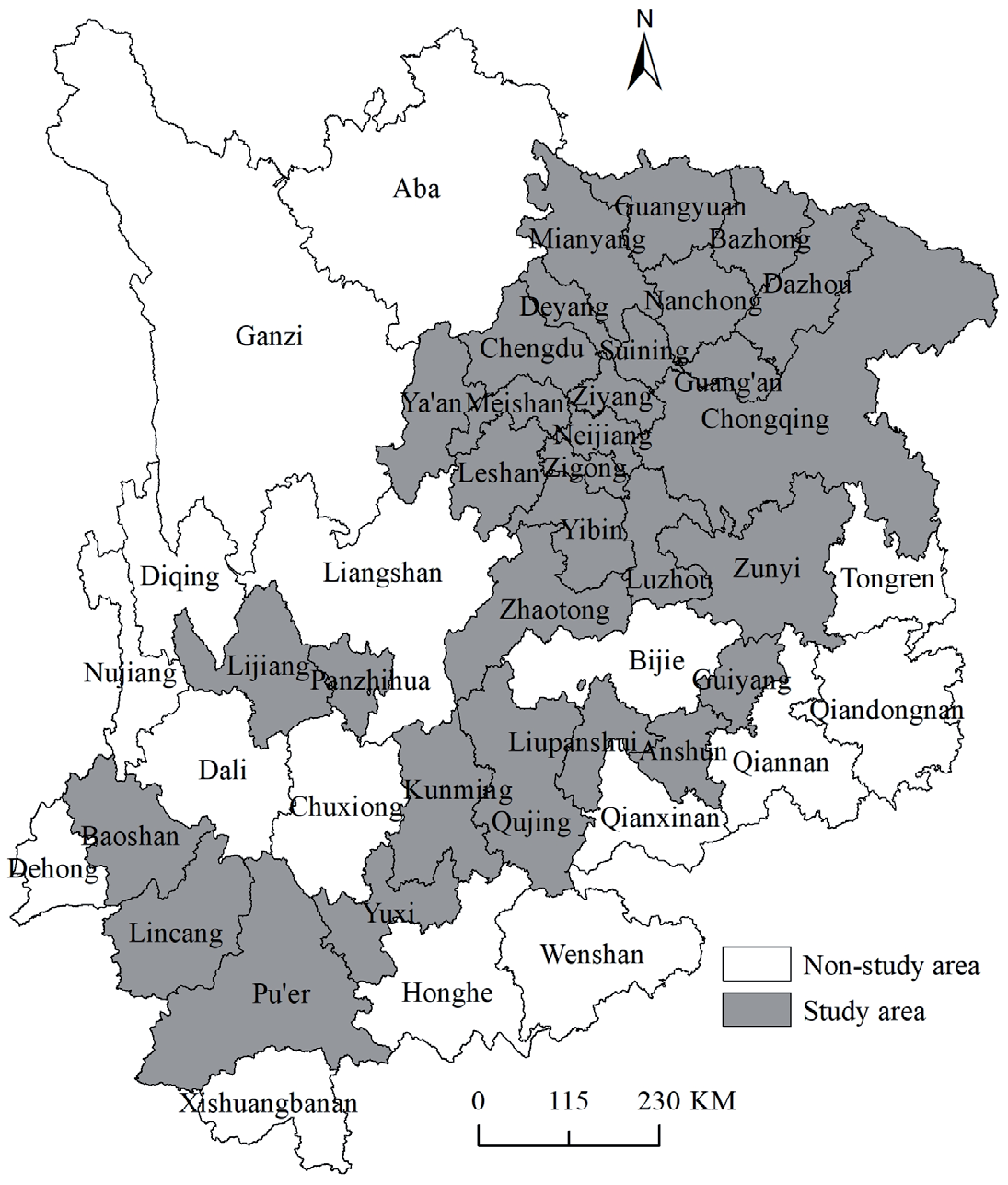
URYR has 47 cities, including 33 prefecture-level cities (PLCs) and 14 autonomous prefectures. Due to the incomplete data publication in autonomous prefectures, data of PLCs are missing to varying degrees in different years. This paper weighs the completeness of the indicators against the number of cities. Then make the decision to choose 2010, 2015 and 2019 as the study years. Because these three years are the years with the largest number of cities when there are the most complete indicators. There are 31 PLCs, including Chongqing, Chengdu, Bazhong, Dazhou, Deyang, Guangyuan, Guang’an, Luzhou, Leshan, Mianyang, Meishan, Neijiang, Nanchong, Yibin, Panzhihua, Suining, Ya’an, Zigong, Ziyang, Guiyang, Anshun, Liupanshui, Zunyi, Kunming, Lijiang, Pu’er, Yuxi, Baoshan, Lincang, Qujing, Zhaotong (Fig. 1).
Data Sources
To reflect ELUPS more accurately, this paper uses the data of PLCs’ municipal districts for research. This type of data mainly comes from the China City Statistical Yearbook (2011, 2016, and 2020). Individual missing data are searched through the corresponding year’s Provincial Statistical Yearbook and the National Economic and Social Development Statistical Bulletin of each PLC, or obtained by interpolating data from adjacent years. However, the Provincial Statistical Yearbook and the National Economic and Social Development Statistical Bulletin of each PLC publishes the city’s data. Therefore, some missing data are calculated by multiplying the city-wide data of the missing year by the proportion of the municipal district data and the city’s data in the adjacent year.
When collating the data, calculate the time series averages of time point indicators such as the number of employed populations. The value of regional GDP, secondary and tertiary industry GDP, fiscal revenue, scientific and education expenditure, and other period indicators are deflated, and 2010 is used as the base period.
Methods
Ecological Level of Urban Production Space Index
Combining the concept of PS and research related to ecologicalization, this paper defines the EPS as sustainable economic development through the green transformation of production mode of PS and the coexistence of environmental protection and economic development. The Chinese government has requirements for industrial greenization, and greenization of production methods. Xi Jinping proposed the theory that lucid waters and lush mountains are invaluable assets [46]. Some scholars proposed that high-quality economic development is structural optimization and rational development [47]. Combining the above viewpoints and the concept of EPS, this paper believes that EPS is inseparable from the guidance of the idea of green development, and green development also requires space and economic support from PS. So, this paper tries to construct the theoretical analysis framework of EPS from three aspects. They are of scalization, structuralization, and greenization (Fig. 2). Among them, scalization and structuralization measure the degree of sustainable economic development. Greenization measures the degree of industrial greenization and greenization of production methods.
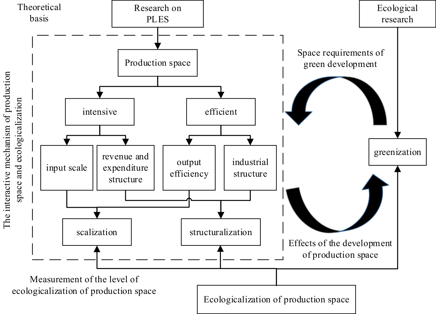
Combined with the theoretical framework of the ecological measurement of PS, the availability of data, and the existing research. This paper constructs an index system for evaluating the ELUPS. It is composed of three aspects, the scalization of production space (SCPS), the structuralization of production space (STPS) and the greenization of production space (GRPS). Among them, the SCPS is measured from 6 indicators from the viewpoint of input scale and output efficiency. The STPS is measured from 4 indicators from the viewpoint of industrial structure and revenue and expenditure structure. The GRPS is measured from a total of 6 indicators from the viewpoint of environmental quality and resource utilization (Table 1). These three aspects are equally important in evaluating ELPS, so this paper uses the equal weight method to calculate the weight of each sub-index.
Extreme Value Method
This paper used the extreme value method to standard each sub-index layer indicator. The formula was:
Positive indicators (indicators with higher values are better):
Negative indicators (smaller values are better indicators):
Among them, Xij' is the jth index value of the ith city after standardization; Xij is the jth index value of the ith city (i = 1, 2, …, n; j = 1, 2, …, m); Max(X:,j) is the maximum value of the jth index in m cities; Min(X:,j) is the minimum value of the jth index in m cities.
Coupling Coordination Model
Based on the coupling degree and coordination degree, the coupling coordination degree can describe the degree of correlation and coordination between the three criterion layers. They are the level of scalization of production space(LSCPS), the level of structuralization of production space(LSTPS) and the level of greenization of production space(LGRPS). The calculation formula of coupling coordination degree is:
Table 1.
Index setting of the ecological level of urban production space.
Where C is the coupling degree of the three criterion layers. T is the coordination degree. L1, L2, L3 are LSCPS, LSTPS and LGRPS respectively. α, β, γ are the undetermined coefficients. Since SCPS, STPS and GRPS are equally important in the EPS, set as α = β = γ = 1/3.
This paper formulates the following standards (Table 2).
The Coefficient of Standard Deviation
The coefficient of variation (CV) can be used to compare the degree of dispersion of the levels of multiple subject indicators at different mean levels. The coefficient of standard deviation (SDC) is the commonly used method in CV. This paper used it to compare the degree of dispersion of ELUPS in the URYR in 2010, 2015, and 2019. Its expression is as follows:
Where Vσt is the SDC in year t; σt is the standard deviation of ELUPS in the URYR in year t; x̅ t is the average value of ELUPS in the URYR in year t.
Spatial Autocorrelation Analysis
Spatial autocorrelation analysis mainly includes global spatial autocorrelation analysis and local spatial autocorrelation analysis. In this paper, Moran’s I and Local Moran’s I are used to analyze whether there is a spatial agglomeration effect on ELUPS in the URYR. Its expression is as follows [48, 49]:
Table 2.
Classification standards of the coupling coordination degree.
Where n is the total number of PLCs; wij is the spatial weight between city i and city j; xti and xtj is ELUPS in city i and city j in year t, respectively; x̅ t is the average ELUPS of all PLCs in year t. s2 is the variance.
Moran’s I can take values between -1 and 1. At a given significance level, If Moran’s I is greater than 0, it means a positive correlation. If it is close to 1, meaning that objects with similar properties cluster together. If Moran’s I is less than 0, it means a negative correlation. If it is close to -1, meaning that objects with different properties cluster together. If Moran’s I is close to 0, meaning that the properties of objects are randomly distributed, or there is no spatial autocorrelation [50]. Positive Local Moran’s I means high-high aggregation or low-low aggregation. Negative Local Moran’s I means low-high agglomeration or high-low agglomeration.
Correlation and Regression Analysis
In this paper, the Pearson correlation coefficient is used to analyze the linear correlation coefficient of ELUPS, per capita GDP, and the number of permanent residents, and the chi square test is carried out. Then the scatter plot is used to fit the regression curve. It will further judge the relationship between ELUPS and per capita GDP and the number of permanent residents
Results and Discussion
Temporal Evolution
Overall Dynamic Evolution Analysis
The descriptive statistics were performed on ELUPS and the criterion layer indicators in 2010, 2015, and 2019 (Table 3). From 2010 to 2019, the overall ELUPS has increased, and the distribution is more concentrated. This is because in the criterion layer indicators, except for LSCPS, LSTPS and LGRPS have generally increased. The distribution of LSCPS and LSTPS are more discrete. The discrete degree of LGRPS is the smallest among the three criterion layer indicators, and it remains the same in the three years. Therefore, the degree of dispersion of ELUPS reduces in the case of equal weights.
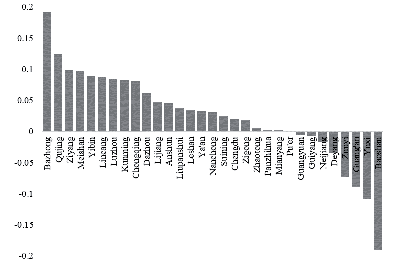
Calculate the difference between ELUPS in 2010 and 2019 (Fig. 3). 22 PLCs’ ELUPS have improved from 2010 to 2019 in the 31 PLCs in the URYR. Bazhong has the highest increase, followed by Qujing, Meishan, Yibin, and other cities. Kunming and Chongqing have a more significant increase than Chengdu. Among the 9 PLCs which ELUPS have declined, Baoshan has the most significant decrease, followed by Yuxi, Guangan, Zunyi, etc. Guiyang has a slight decline.
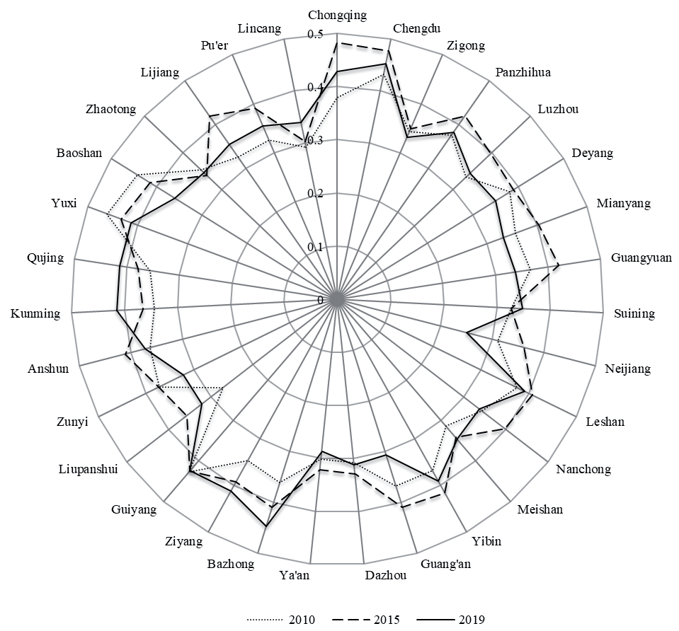
Formula (3)-(5) are used to calculate the coupling coordination degree. PLCs of moderate coupling coordination degree in 2010 include Chengdu, Guiyang, Yuxi, and Baoshan. Others have low coupling coordination degree. In 2015, Chongqing, Chengdu, Panzhihua, Mianyang, Guangyuan, Leshan, Yibin, Guang’an, Bazhong, Guiyang, Anshun, Yuxi, Baoshan, and Lijiang have moderate coupling coordination degree. In 2019, PLCs of moderate coupling coordination degree are Chongqing, Chengdu, Bazhong, Ziyang, Guiyang, Kunming, Qujing, and Yuxi. Generally, only Chengdu, Guiyang, and Yuxi are in moderate coupling coordination degree state for three years (Fig. 4).
Spatial Evolution
Spatial Evolution of LSCPS, LSTPS, and LGRPS
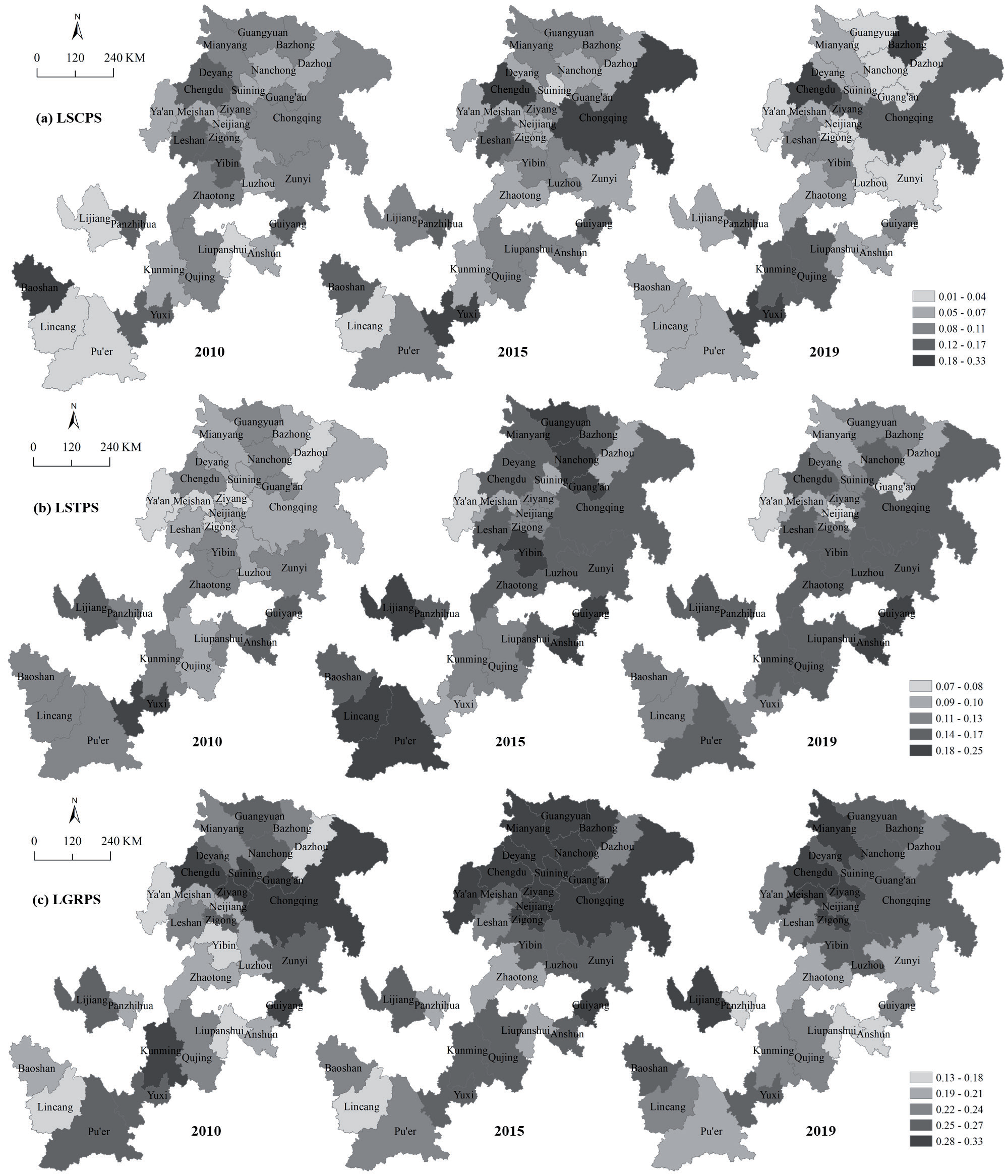
In this paper, LSCPS, LSTPS, and LGRPS in 2010 were divided into 5 levels by the natural discontinuous point grading method in ArcGIS 10.2 software. Then the corresponding indices in 2015 and 2019 were graded according to this interval.
From the perspective of spatial distribution, in 2010, cities with higher LSCPS were scattered among Sichuan Provinces, Yunnan Provinces, and Guizhou Provinces, mainly including Baoshan, Chengdu, Deyang, Leshan, Yibin, Guiyang, Yuxi, and Panzhihua. The cities with medium LSCPS were mostly zonal distributed in the north and east of the study area, including Chongqing. This is because the annual average urban construction land area (AAUCLA) of Chongqing in 2010 reached 774.5 km2, which is about 1.8 times of Chengdu, about 8.3 times the AAUCLA of 31 PLCs. Other indicators related to LSCPS, such as the added value of the secondary industry in the municipal area, the number of employees, the added value of the tertiary industry, the number of employees, and scientific and educational expenditures are less than 1.5 times of Chengdu, and the fiscal revenue of the municipal district is smaller than that in Chengdu. Therefore, the LSCPS of Chongqing in 2010 was only moderate. The cities with lower LSCPS were mainly concentrated above and below the Chengdu-Chongqing connecting line, and in the west of the study area, including Kunming. In 2010, the AAUCLA of Kunming was comparable to Chengdu, and it was about 4.4 times the AAUCLA of the 31 PLCs. But the values of other indicators related to LSCPS were smaller than that in Chengdu. In addition to Kunming, Luzhou, Nanchong, Suining, Neijiang, and Liupanshui also had a significant AAUCLA and the average performance of other indicators. These made lower LSCPS. Compared with other cities, the cities such as Anshun, Ya’an, Dazhou, Pu’er, Lijiang, and Lincang had many lower levels of indicators. The indicators were the added value of the secondary industry, the number of employees, the added value of the tertiary industry, the number of employees, scientific and educational expenditures, and fiscal revenue. It made lower LSCPS in these cities.
Table 3.
Descriptive statistics of ELUPS and the criterion layer indicators in the URYR in 2010, 2015 and 2019.
In 2015, the cities with the highest LSCPS were Chengdu, Chongqing, and Yuxi. Cities with higher LSCPS were scattered among Sichuan Provinces, Yunnan Provinces, and Guizhou Provinces, mainly including Leshan, Guiyang, Panzhihua, and Baoshan. Cities with medium LSCPS primarily concentrated in the north and south of the study area. Cities with lower LSCPS were zonal distributed between Sichuan Provinces, Yunnan Provinces, and Guizhou Provinces, especially the above and below the Chengdu-Chongqing connecting line. In 2019, LSCPS were locally concentrated in space. Cities with higher LSCPS were mainly concentrated on the Chengdu-Chongqing connecting line and the Yuxi-Qujing connecting line. Cities with lower LSCPS were zonal distributed in the west of the study area and above and below the Chengdu-Chongqing connecting line (Fig. 5a).
Combined with the composition indicators of LSCPS, it is possible to find that the cities with lower LSCPS had a lower economic scale than other cities. Therefore, in general, the cities in the west of the study area and the above and below the Chengdu-Chongqing connecting line should improve the economic scale level.
In 2010, cities with a higher LSTPS were scattered between Yunnan Province and Guizhou Province, mainly including Yuxi, Lijiang, Anshun, and Guiyang. Cities with a medium LSTPS were primarily zonal distributed in the study area and around the junction of Sichuan Province, Yunnan Province, and Guizhou Province. Cities with lower LSTPS were mainly zonal distributed in the north of the study area, including most cities in the Chengdu-Chongqing economic circle (CCEC). In 2015 and 2019, cities with medium and higher LSTPS accounted for the vast majority, and they were zonal distributed in the study area. Cities with lower LSTPS were mainly scattered in Sichuan Province. It primarily included Neijiang, Guang’an, Ya’an, Meishan, Dazhou, and Mianyang in 2019 (Fig. 5b).
Combined with the composition indicators of LSTPS, compared with other cities, cities with lower LSTPS had a lower proportion of fiscal revenue in GDP and scientific and educational expenditures in GDP. For example, in 2019, the average proportion of fiscal revenue in the GDP of 31 PLCs was 3.12%, and the average proportion of scientific and educational expenditures in the GDP of 31 PLCs is 1.44%. But Ya’an, one of the cities with lower LSTPS, is 0.89% and 1.02%, respectively.
In 2010, cities with higher LGRPS were mainly zonal distributed in the southwest, east of the study area, and the Chengdu-Chongqing connecting line and the above of it. Cities with lower LGRPS were mainly zonal distributed in the west and middle of the study area. In 2015, cities with higher LGRPS were mainly zonal distributed in the north and east of the study area and around Kunming. Cities with medium and lower LGRPS were primarily concentrated on the west side of the study area. The rest of the cities were primarily scattered around the junction of Sichuan Province, Guizhou Province, and Yunnan Province. In 2019, cities with higher LGRPS were primarily zonal distributed in the north of the study area. Cities with medium and lower LGRPS were primarily concentrated in the south and middle of the study area, especially around the border of Sichuan Province, Yunnan Province, and Guizhou Province (Fig. 5c).
Combined with the composition indicators of LGRPS, most cities with lower LGRPS mainly suffer from lower resource utilization efficiency, and some cities have both lower environmental quality and lower resource utilization efficiency, such as Liupanshui and Panzhihua, in 2019.
Spatial Evolution of ELUPS
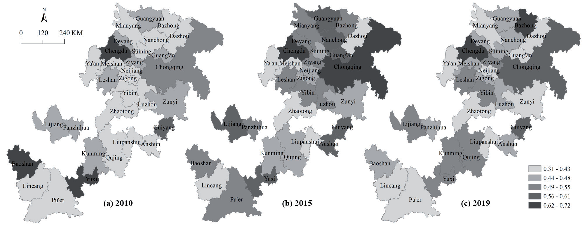
ELUPS in 2015 were divided into 5 levels by the natural discontinuous point grading method in ArcGIS 10.2 software. Then ELUPS in 2010 and 2019 were graded according to this interval. Judging from the number of cities corresponding to each level, ELUPS in 2010, 2015, and 2019 were significantly differentiated. In 2010 and 2019, the number of cities corresponding to each grade from high to low presented a vase shape of “small first and then large”. In 2015, it appeared in the form of a “small at two ends and big in the middle”.
From the perspective of spatial distribution, in 2010, cities with higher ELUPS were scattered in the east, west, south, and north of the study area, including Yuxi, Baoshan, Chengdu, and Guiyang. The cities with lower ELUPS were zonal distributed in the study area. In 2015, cities with higher ELUPS were mainly concentrated in provincial capital cities and municipalities directly under the Central Government or their surrounding areas. They showed a spatial pattern of “high in the northeast and southwest, and low in the middle”. In 2019, cities with higher ELUPS were scattered in the north and east of the study area, including Chengdu, Bazhong, Chongqing, and Guiyang. Cities with medium ELUPS were mainly concentrated in Leshan and Yibin areas and around Kunming. Cities with lower ELUPS were mainly zonal distributed in the west of the study area, around Guiyang, and in the above and below the Chengdu-Chongqing connecting line. This is similar to the spatial distribution of LSCPS in 2019 (Fig. 6).
Spatial Correlation
The ArcGIS 10.2 software was used to construct a spatial weight matrix using shared boundaries and nodes, and the global Moran’s I index and related indicators of ELUPS in the URYR in 2010, 2015, and 2019 were calculated. The results show that the global Moran’s I indices were small, and the Z values of the normal statistic were less than the critical value of 1.96 at the 0.05 confidence level in 2010, 2015, and 2019. Therefore, it can be considered that from 2010 to 2019, there was no significant spatial correlation between ELUPS in the 31 PLCs in the URYR, and they were randomly distributed. It means that ELUPS in the PLCs did not affect each other.
This paper further analyzed the relationship between ELUPS in 31 PLCs in the URYR in geographic space. It tested their spatial correlation and convergence trend in local areas. The spatial weight matrix was the same as above. Then, conducted local spatial autocorrelation analysis of ELUPS in the URYR in 2010, 2015, and 2019 in ArcGIS 10.2 software. The results show that only significant high-low agglomeration or low-high agglomeration occurred in 2010, 2015, and 2019. It indicated that PLCs with higher ELUPS did not have a radiation effect on surrounding PLCs.
Influencing Factor Analysis
The paper compared the SDCs of the criterion layer indicators of ELUPS in the URYR in 2010, 2015, and 2019 (Table 3). It can be seen that LSCPS had the largest SDC among the three criterion layer indicators in the three years. The second was LSTPS. The last was LGRPS. This means that when the three criterion layer indicators have equal weights, LSCPS is the main factor leading to the difference in ELUPS of each PLC, followed by LSTPS. This confirms the conclusion that the spatial distribution of ELUPS was similar to the spatial distribution of LSCPS. In addition, LSCPS was mainly reflected by the level of the economic scale. This paper conjectures that the spatial differences in ELUPS in the URYR in 2010, 2015, and 2019 were affected by the level of the economic scale.
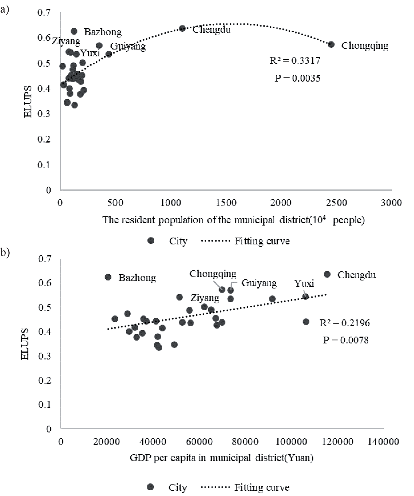
To test the above conjecture, this paper calculated the linear correlation coefficients between ELUPS, GDP per capita, and resident population of 31 PLCs in the URYR (Table 4). The result shows that except the correlation coefficient between ELUPS and the number of permanent residents in 2010 was not significant, other correlation coefficients were two-tailed significant at the 0.05 significance level. It means that there is a significant positive linear correlation between ELUPS and the average resident population and per capita GDP of 31 PLCs.
This paper made scatter plots on ELUPS, average resident population, and per capita GDP of 31 PLCs in 2019 (Fig. 7a), and preliminary fitted trend line (Fig. 7b). The trend line equations were all significant. In 2019, with the increase in the average resident population, the change in ELUPS was generally parabolic. It will reach the highest point when the number of permanent residents is about 15 million. ELUPS and the per capita GDP were a flat linear relationship. That is, under the same other conditions, the higher the per capita GDP, the higher ELUPS.
Conclusions
Based on the existing data and related research, this paper established an index system for evaluating ELUPS in the URYR. Then this paper used the equal weight method to determine the weight of each index, and analyzed ELUPS from the perspective of time and space. The conclusions are as follows:
Table 4.
Linear correlation index of ELUPS, resident population, and GDP per capita in 31 PLCs.
| Index | 2010 | 2015 | 2019 |
|---|---|---|---|
| Average resident population of the municipal district (104 people) | 0.25 | 0.60** | 0.45* |
| GDP per capita in municipal district (Yuan) | 0.47** | 0.42* | 0.47** |
Fig. 7.
Scatter diagram and fitting trend of ELUPS, resident population a), and GDP per capita b) in 31 PLCs.
(1) From 2010 to 2019, most of the 31 PLCs in the URYR had improved ELUPS. Bazhong increased the most, and Baoshan decreased the most. The mutual influence between cities was weak. The overall agglomeration effect was not formed.
(2) From 2010 to 2019, the degree of correlation and coordination between LSCPS, LSTPS and LGRPS are low. From the point of view of the index composition, it is mainly caused by the insufficient level of economic development.
(3) In 2019, LSCPS in the URYR showed a spatial pattern of partially prominent, lower in the west of the study area, above and below the Chengdu-Chongqing connecting line. LSTPS presented a spatial pattern of higher overall and lower sporadic. LGRPS was higher in the north of the study area, and lower in the south and middle of the study area. The changes in the three criterion layer indicators made ELUPS present a spatial pattern of partially prominent, lower in the west of the study area, around Guiyang, above and below the Chengdu-Chongqing connecting line.
(4) LSCPS was the main factor leading to the difference in ELUPS of various PLCs, followed by LSTPS. There was a significant positive linear correlation between ELUPS and the average resident population and per capita GDP in 31 PLCs. If other conditions remain unchanged, cities with a permanent population of about 15 million and cities with higher per capita GDP are more conducive to ELUPS.
The research shows that ELUPS in the URYR presented a phenomenon of stratification. Higher level ELUPS cities had insufficient driving force. The URYR had weak inter-city influence. In addition, the coupling coordination degree between economic development and environmental conditions in ELUPS is low. According to the spatio-temporal variation characteristics of indicators and the analysis results of influencing factors, under the condition that there is little difference in the LGRPS, the expansion of UPS scale, the optimization of structure and the agglomeration of population will bring about the improvement of the ELUPS. In general, the problems of EPS’s development in the URYR is mainly caused by economic development. Similar conclusions have been reached in other studies of green development [51-53]. The polarization of urban scale in the URYR distorts the hierarchical structure of the urban system, and it squeezes the vast number of small and medium sized cities’ capacity to undertake the resource. It weakens the potential of the Chengdu-Chongqing dual core spillover effect [54]. Therefore, promoting high-quality development in the URYR is a critical way to improve ELUPS in the URYR.
First of all, the URYR should focus on reducing the phenomenon of urban stratification. All PLCs should implement new development concepts. Develop their economies according to local conditions. Support local enterprises to become bigger and stronger, and find ways to integrate into the construction of the CCEC. Leverage the relationship with the higher ELUPS cities to develop.
Secondly, the URYR should use the CCEC to strengthen the connection between cities continuously. At present, the construction of the CCEC focuses on improving the development level and comprehensive competitiveness of the central city of Chongqing and Chengdu, and promoting the interaction between cities inside and outside the economic circle. So far, the government published many documents to promote the construction of the CCEC, such as the “Three year action plan for the integrated development of transportation in the CCEC (2020-2022)”, the “Coordinated action plan for promoting the green, low carbon and high-quality development of Sichuan-Chongqing energy”, and “Some policies and measures to support the healthy development of market entities in CCEC” et cetera. Promote the joint development of cities such as the integration of Chengde and Meizi, the Tongnan-Anyue lemon industry cluster, the Yongchuan-Luzhou modern agriculture demonstration zone, and the Sichuan-Guizhou-Chongqing demonstration zone. However, how to promote more urban interaction and how to establish cooperative links with cities in the middle and below reaches of the Yangtze River needs to be further explored.
The limitations of this paper are as follows:
(1) The index system constructed to evaluate ELUPS in the URYR is based on the urban spatial scale. It causes the accuracy of the evaluation index to be insufficient.
(2) The severe lack of data in some cities leads to flawed real time and comprehensive analysis. Therefore, it is a long term and complex academic topic to identify the PLE and collect relevant data for evaluation, which deserves further in depth study.