

Introduction
The expanding scope and intensity of human activities have directly or indirectly subjected regional ecosystems to varying degrees of stress due to anthropogenic disturbances [1, 2]. This damages ecosystem structures, processes, and functions, thereby leading to multiple uncertain ecological risks [3, 4]. As land use reflects the interaction of human activities and the environment, landscape ecological risk (LER) assessment based on land use and cover change (LUCC) is a vital tool to measure the effects of human activities on the ecological environment [5-7]. It is also a key research element for regional environmental protection and management [8-11]. Therefore, based on land use, LER assessment models that focus on the comprehensive ecological risk effects of specific landscape combinations, spatial patterns, and their changes can be introduced [12-17]. Regional LER assessments and scientific studies on its spatiotemporal variations are important to construct a regional “ecological civilization”, restore ecosystems, and provide early warnings of LER [12, 13, 17-23]. In recent years, with comprehensive research on global changes and ecological risks, ecosystem damage caused by changing land use has received growing attention from researchers and environmental managers, and studies on LER assessment have become a popular research topic [24-44]. Our review of studies on LERs revealed that previous research was focused on macro, meso, and micro scales, such as coastal zones, regions, water bodies, urban clusters, provinces, municipalities, counties, townships, nature reserves, and mining areas [45-61]. Moreover, previous studies have explored the LER patterns of plateaus, mountains, valleys, plains, basins, and other landform types [48, 62-64], with research primarily focusing on urban, oasis, grassland, wetland, arable land, and unused lands [24, 47, 65-68]. In terms of research methodology, landscape pattern index, kriging interpolation, entropy analysis, ecosystem services value, exposure–response, and other GIS-based spatial analyses are the most common methods of LER assessment [4, 8, 48, 54, 69-71]. Due to global climate and environmental changes [72-75], achieving dynamic monitoring of land use/cover based on GIS and RS technology to quantitatively investigate the spatial differentiation of landscape ecological risks in a specific region has become a new hotspot and research direction for the optimal allocation and sustainable development of landscape patterns [76-80]. Regarding the analysis of drivers of LER, conventional analytical techniques, such as correlation analysis, multiple linear regression, geographically weighted regression, and geographical detector, remain the most common approaches [53, 56, 81-86]. In summary, since the concept of landscape ecological risk assessment was proposed, its underlying theory, analytical methods, structural frameworks, and research paradigms have been extensively explored.
Research outcomes of landscape ecological risk assessment based on land use changes have also been continuously enriched and updated [8, 47, 49, 50, 52, 84, 87, 88]. Nonetheless, the current research in this field remains in the initial and exploratory phases. First, ecological receptors are primarily single risk sources and receptors, and there has been limited work on landscape ecological risks and their spatial patterns via coupling response mechanisms with enviro–social systems [24, 81, 87, 89]. Second, previous studies mainly emphasized landscape ecological risks and their spatial patterns, while systematic and comprehensive analyses of the spatiotemporal variation characteristics and the drivers of LERs have been seldom included. Even though existing studies have also explored the drivers of LER, the previous research methods for the drivers mainly focused on traditional statistical analysis to examine the linear relationship between independent variables and response variables. Due to the spatial heterogeneity of landscapes, the relationship between LER and the responses of different drivers is very complex and nonlinear. Therefore, it is urgent to introduce newly developed machine learning algorithms, such as the boosted regression trees (BRT) model, to quantitatively identify the effects of natural factors and human activities on response variables and their nonlinear relationships. The BRT model is a novel machine learning approach that can visually represent complex nonlinear relationships, automatically handle the interaction effects among predictor variables, efficiently achieve excellent predictive performance, and greatly overcome overfitting [90, 91]. However, little is known about the studies in landscape ecology that have been used to fit and characterize LER and the interactions of different predictor variables. Therefore, to overcome this knowledge gap, this study used the BRT model to systematically disentangle the effects of different drivers on LER. Moreover, the regional scopes of existing studies have mainly been water bodies and cities, with fewer relevant investigations in ecological “security barriers” or eco-sensitive regions (e.g., Qinling-Daba Mountains). This makes it difficult to effectively guide LER assessment and risk prevention in such regions.
Ankang City is situated in the hinterland of the Qinling-Daba Mountains region; 40% and 60% of its land area consists of the Qinling Mountains and the Daba Mountains, respectively, which are closely connected by its geographical location. In addition, Ankang has unique advantages in terms of biological resources and excellent ecosystems. Meanwhile, it is not only a special area with an extremely fragile and sensitive ecological environment in the Qinling-Daba Mountains region, but also a critical area that needs urgent protection and great attention from human beings. The Qinling-Daba Mountains, where Ankang City is located, represent a key geographical transition zone and watershed for northern and southern China in terms of geography and climate. It is a key ecological security barrier, playing a vital role in climate regulation, soil and water conservation, and habitat maintenance [92]. With continuous socioeconomic development and extensive transformation, the challenges between the human population and the carrying capacity of the environment in Ankang are becoming increasingly prominent. This has led to multiple environmental problems, such as excessive land cultivation, increased forest destruction, frequent natural disasters, severe soil erosion, and a sharp biodiversity decline [93-95]. Thus, there is an urgency for environmental protection in Ankang. As Ankang is the most typical and sensitive area in the Qinling-Daba Mountains region [96-98], studying spatiotemporal patterns, variations, and drivers of the LERs is of great practical significance for the environmental conservation and protection of the Qinling Mountains in China. This would not only enrich the ecological understanding of eco-sensitive areas in China, but also provide vital support for landscape planning and zoning management decisions. Thus, the objectives of this study are as follows: (1) to construct a LER assessment model based on land use and land cover; (2) to investigate the spatiotemporal variation characteristics of LERs through spatial statistical methods; and (3) to quantify the drivers for LERs using the BRT model.
Materials and Methods
Overview of the Study Area
Ankang is located in the area ranging from 31°42′24″ to 33°50′34″N and 108°00′58″ to 110°12′00″E in the hinterland of the Qinling-Daba Mountains, on the banks of the Hanshui River, in the southeast of Shaanxi Province, bordering Wudang (Hubei Province) in the east, Hanzhong (Shaanxi Province) in the west, the northern slope of the Bashan Mountain in the south, and the main ridge of the Qinling Mountains in the north. Hanshui River-Chihe River-Yuehe River-Hanshui River mark is the geographical boundary between Qinling and Daba mountains, and the landform is characterized by “high mountains in the north and south and a valley basin in the middle.” The elevation is the lowest (170 m above sea level) on the right bank of the Hanshui River, at the border between Baihe County and Hubei Province, and the highest (2964.6 m above sea level) in Dongliang in the Qinling Mountains. Ankang covers a land area of 2.35 × 10⁴ km2, with one district and nine counties under its jurisdiction and a resident population of 2,668,900 individuals. The region has a subtropical continental monsoon climate, with abundant light and a humid, mild climate. There are four distinct seasons, with abundant rainfall and a long frost-free period. The mean annual temperature (MAT) is approximately 15ºC-17ºC, the MAT difference is approximately 22ºC-24.8ºC, the mean annual precipitation (MAP) is around 1,050 mm, and the MAP period is 94 days. The mean annual crop-growing period is 290 days, with a mean annual frost-free period of 253 days. The mean annual sunshine duration is 1,610 h, with a total annual solar radiation of 4.435 × 10⁵ MJ·m−2. With a dense network of rivers, water resources in the territory are extremely abundant. The major vegetation types include subtropical evergreen broad-leaved, deciduous broad-leaved, and mixed forests of both types. With an extensive area of woodland, the city enjoys the reputation of being the “national forest city” and the “natural biological gene bank”.
Data Sources and Data Processing
The ecological and environmental protection planning database, general land use planning database, and socioeconomic statistical yearbook data originated from the website of Ankang Municipal People’s Government (https://www.ankang.gov.cn/). The 30 m× 30 m land use and land cover data for 2000, 2010, and 2020 developed by the National Geomatics Center of China were acquired from the website of GlobeLand30 (http:// www.globallandcover.com/). The 90 m× 90 m elevation, slope, and slope of aspect calculated by the 2010 digital elevation model (DEM) were obtained from the Geospatial Data Cloud platform (http://www.gscloud. cn). The 1000 m × 1000 m data on landform type during 1980-2009 were acquired from the Resource and Environment Science Data Center, Chinese Academy of Sciences (https://www.resdc.cn/). The 1000 m × 1000 m data on normalized difference vegetation index (NDVI), MAT, MAP, aridity index, GDP, population density (PD), night lights, and soil erosion for 2000, 2010, and 2020 were obtained from the Resource and Environment Science Data Center, Chinese Academy of Sciences (https://www.resdc.cn/). The 1000 m × 1000 m data on soil types during the Second National Soil Survey were obtained from the National Tibetan Plateau Data Center (https://data.tpdc.ac.cn/). The 1000 m × 1000 m data on soil properties during 2010-2018 were obtained from the National Earth System Science Data Center (http://www.geodata.cn/). Soil properties included soil texture (ST), soil bulk density (SBD), coarse fraction (CF), soil thickness (STH), soil organic carbon (SOC), soil total nitrogen (STN), soil total phosphorus (STP), soil total potassium (STK), pH, and cation exchange capacity (CEC). In the present study, all spatial data was pre-processed in ArcGIS 10.8 software. Quantitative analysis of drivers was run in R 4.0.3 software.
Research Methodology
Division of Risk Units
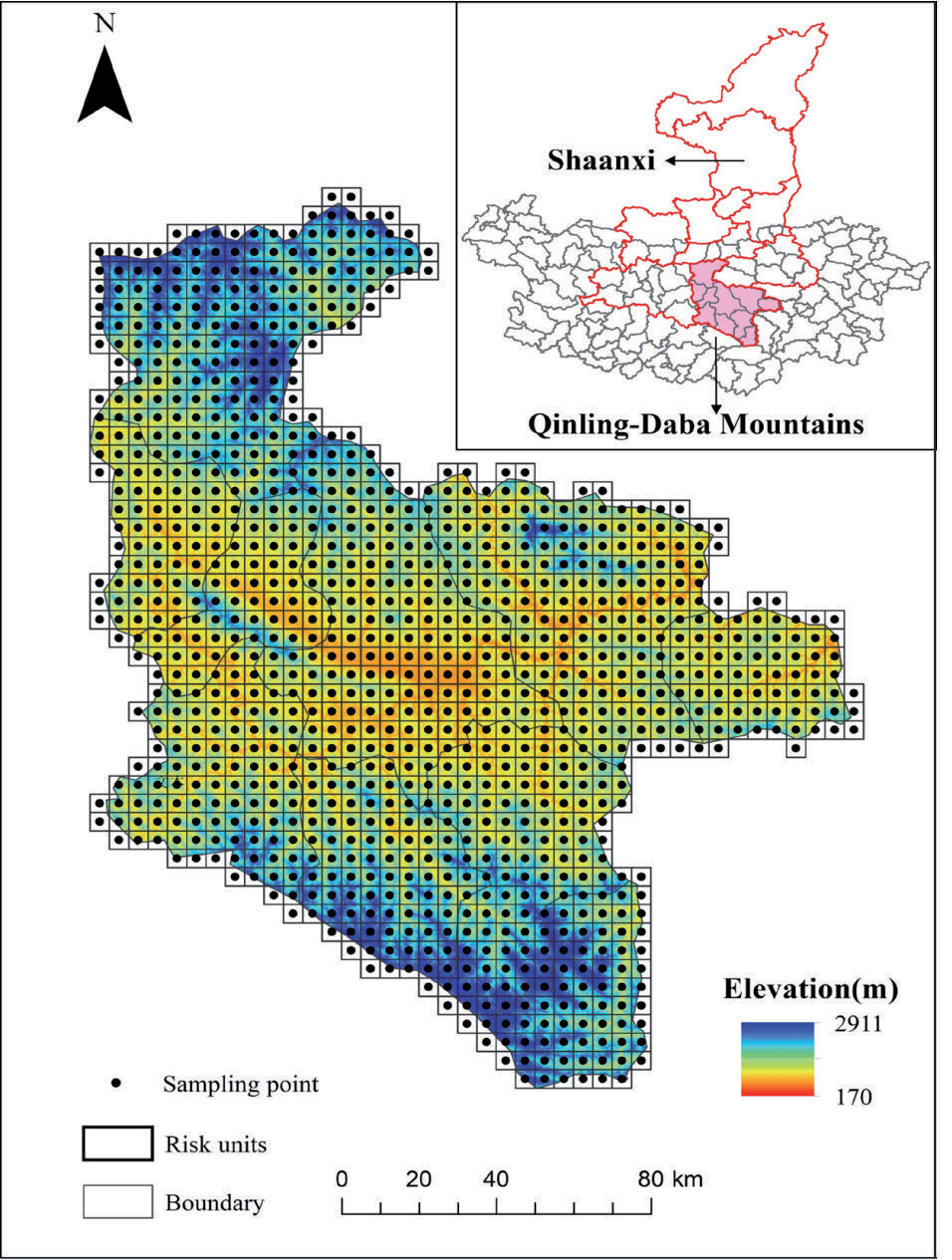
Using the ArcGIS 10.8 software, the study area was divided into a considerable number of grids for raster data analysis. Referring to the national grid GIS standard “Geographic Grid” (GB12409-2009) and landscape ecology principles, the grid size was generally sampled at 2-5 times the average patch area. After comprehensive consideration of the study area, topographic features, and landscape spatial heterogeneity, the 5 km × 5 km grid was finally selected to sample the study area at equal spacing (Fig. 1) following repeated tests. Each grid was coded for division into 1037 landscape ecological risk units, of which 921 were valid grids (i.e., the country area falling within the ith grid was >50% of the grid area). Then, the center point of the valid grid cell was selected as the sampling point to represent the landscape ecological risk value within the grid, and the landscape type and ecological risk units were input into FRAGSTATS 4.2 to derive the ecological risk index of each ecological risk unit. The center point of the risk unit was used as the sample for ordinary Kriging interpolation analysis. Finally, the spatial distribution pattern of ecological risks in the study area was obtained.
Construction of the Landscape Ecological Risk Index
The landscape index method is a widespread quantitative research approach in ecology and geography that describes changes in landscape patterns and ecological risks by constructing multiple landscape indices for integrated analysis. The construction of the landscape ecological risk index (LERI) not only helps to identify the extent of natural and anthropogenic disturbances to ecosystems [65, 67, 99, 100], but also measures the resilience of different ecosystems in the region [24, 39]. In the present study, we selected the landscape fragmentation index (Ci), landscape separation index (Si), landscape dominance index (Ki), landscape disturbance index (Ui), landscape vulnerability index (Ei), and landscape loss index (Ri), which represent the degree of fragmentation of the landscape type, the degree of separation between different patches in the landscape type, the degree of dominance of the landscape type, the degree of disturbance of the landscape type, the magnitude of resistance of the landscape type to withstand external disturbances, and the degree of ecological loss of the landscape type [14, 23, 24, 39, 43, 53, 63, 67, 69, 99, 101], respectively. These were based on the area and number of patches in constructing a LERI for characterizing the spatial distribution pattern and determining the spatiotemporal variation characteristics of LERs in Ankang. The landscape pattern index, calculation method, and ecological interpretation are referenced in the previous literature [23, 24, 39, 43, 53, 63, 67, 69, 99, 101].
Spatial Statistics
Spatial Autocorrelation Analysis
Spatial autocorrelation analysis can be used to test whether spatial variables are significantly correlated with adjacent regions at a given location, and their spatial dependence properties are primarily measured and obtained through global and local spatial autocorrelation indices [55]. Global spatial autocorrelation (global Moran’s I) measures the overall degree of spatial dependence and distribution pattern of an attribute based on the element’s location and value. Local spatial autocorrelation (local Moran’s I) reflects the degree of correlation or similarity between each spatial unit and its neighboring spatial units for a certain attribute value in the local space and its significance.
The global spatial autocorrelation index was calculated as follows [102]:
The local spatial autocorrelation index [89]:
where n denotes the total number of elements, xi represents the observed value of the ith element, x̅ denotes the average value of xi, and Wij denotes the binary adjacency spatial weight matrix between elements i and j, indicating the relationship of spatial adjacency. At a certain significance level, global Moran’s I>0 indicates that ecological risks exhibit a spatial positive correlation: the greater the value of global Moran’s I, the stronger the spatial correlation. In global spatial autocorrelation, global Moran’s I = 0 suggests that ecological risk is randomly distributed, while global Moran’s I<0 indicates that LERs exhibit a negative spatial correlation; the smaller the value of global Moran’s I, the greater the spatial variability. In local spatial autocorrelation, local indicators of spatial association (LISA) clustering maps are normally used to visualize whether there are significant high–high and low–low spatial clustering areas of ecological risk observations in a local area. Local Moran’s I>0 indicates spatial aggregation of similar values (high or low) around ecological risk in the region. Local Moran’s I = 0 indicates that the spatial aggregation characteristics of ecological risks are randomly distributed. Local Moran’s I < 0 indicates the spatial aggregation of non-similar values of ecological risks.
Geostatistical Analysis
Spatial analysis of the ecological risk indices of regional landscapes was performed using the semi-variance function of the geostatistical variance function. The specific formula is as follows [46]:
where γ(h) denotes the semi-variance function, h represents the sample spacing, and N(h) is the number of sample point pairs at h sampling spacing. Z(Xi) and Z(xi+h) are the observed values of the ecological risk index at the spatial locations xi and xi+h, respectively. In the present study, the theoretical model of the geostatistical semi-variance function for the study area was fitted and cross-validated using GS+9.0. The optimal model and the corresponding parameters were selected. Spatial interpolation of the corresponding parameters was conducted in ArcGIS 10.8 using the ordinary kriging method to characterize the spatiotemporal variation patterns of LERs.
Standard Deviation Ellipse Analysis
Standard deviation ellipse analysis is a spatial statistical method that quantitatively describes the overall characteristics of the spatial distribution of geographic elements. It can quantitatively reveal the centrality, spreading, direction, spatial pattern, and other multifaceted characteristics of the spatial distribution of geographic elements from global and spatial perspectives [103]. Its primary parameters were calculated using the following formulas:
where xi and yi denote the coordinates of the x and y axes of element i, respectively; tanθ denotes the azimuth of the ellipse; [1] denotes the gravity center of the element; and n is the total number of elements. SDEx and SDEy are the coordinate lengths of the x and y axes, respectively. x͂ i and y͂ i denote the coordinate deviations of the x and y coordinates of element i from the gravity center of the ellipse [49], respectively. σx and σydenote the standard deviations along the x and y axes, respectively.
BRT Model
BRT is a relatively new machine learning method for classification and regression. It integrates the strengths of both regression trees and boosted algorithms [104]. BRT models can handle different types of predictor variables, accommodate missing data, transform data, eliminate outliers, fit complex nonlinear relationships, identify significant variables, and automatically handle interactions among variables. Therefore, BRT models outperform most common machine learning and conventional modeling approaches, such as random forest and support vector machines, in terms of prediction [91]. Before running the BRT model, the following four important parameters must be set to ensure the stability of the model operation: family, tree complexity, learning rate, and bag fraction. After repeated tests, the four primary parameters of the BRT model were set as follows: family = “gaussian,” tree complexity = 10, learning rate = 0.001, and bag fraction = 0.750. The BRT model automatically cross-validated the simulation results during the run, and 75% of the data were automatically extracted as the training set and the remaining 25% as the testing set each time to ensure optimal model prediction results. To illustrate the validity of the BRT model, tenfold cross-validation was used to evaluate the predictive performance using mean absolute error (MAE), root mean square error (RMSE), and coefficient of determination (R2). The boosting algorithm adopts a repeated iterative technique to gradually increase decision trees to generate the optimal model, which makes the BRT model an ideal machine learning tool for this present study. In the present study, the BRT model was run in RStudio 4.0.3, and two library packages, namely “dismo” and “gbm”, were called to build the BRT model for identifying and filtering the drivers of LERs.
Results
Land Use Type Changes
Land use structural changes and the land use transition matrix in Ankang during 2000-2020 are shown in Fig. 2 and Table 1, respectively. During 2000-2020, among land use types in the study area, the areas of cropland, woodland, and unused land decreased gradually, whereas the areas of grassland, water bodies, and construction land increased significantly. Woodland and cropland were the primary land types that were converted in the study area, measuring 863.02 and 565.36 km2, respectively. Woodland was primarily converted to cropland, grassland, water, and construction land, while cropland was primarily converted to woodland, grassland, and construction land. In addition, the areas converted to woodland and cropland were 742.77 and 515.59 km2, respectively, with these areas being smaller than the areas converted to other land uses, resulting in a decrease in the overall area. The increase in unused land was primarily due to the conversion of woodland and grassland. Cropland was largely supplemented by woodland, grassland, and construction land (land reclamation). Meanwhile, the increase in woodland was mainly due to conversion from cultivated land and grassland. Water bodies were primarily supplemented by woodland and grassland. The increase in construction land mostly resulted from cultivated land, grassland, and water bodies. Water bodies were primarily converted to woodland, grassland, and cropland, and the construction land was primarily supplemented by cropland, grassland, and water bodies. These results suggested that urbanization and economic development were the dominant factors in land use changes in this region.
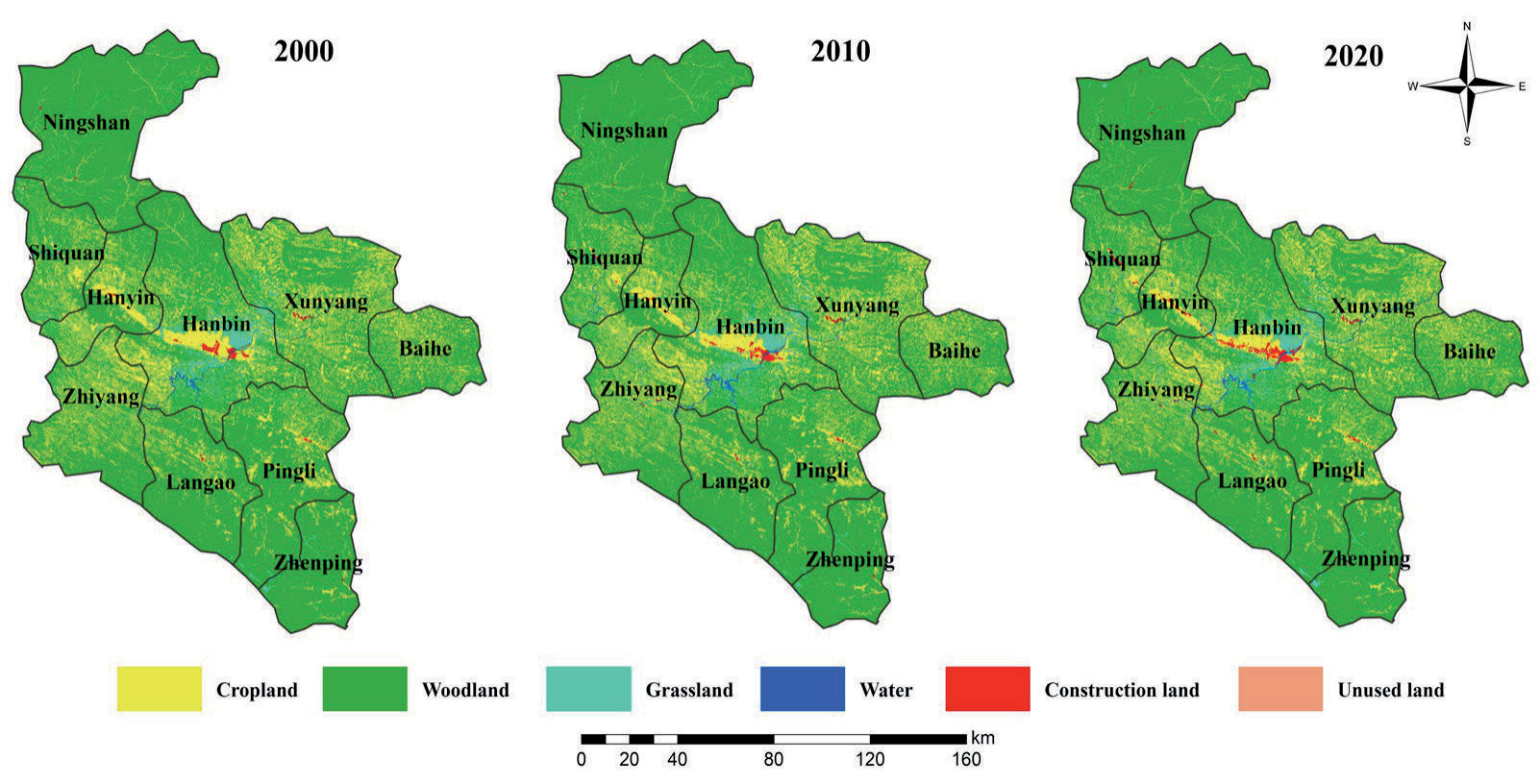
Table 1.
Landscape type transfer matrix in the study area during 2000-2020.
Landscape Ecological Risks
The number and area of patches of different landscape types in the study area for the three periods were calculated using the type and landscape level in FRAGSTATS 4.2, and then the landscape indices for different landscape types were derived using the calculation method in Table 2. From 2000 to 2020, the decrease in cultivated land area and increase in the number of patches in the study area resulted in a gradual increase in the fragmentation, separation, dominance, disturbance, and loss of landscape. The area of woodland declined significantly, and the number of patches increased and then decreased, resulting in a fluctuating trend of an increase before a decrease in the five landscape indices. The area of grassland increased gradually, while the number of patches decreased sharply. This may be attributed to the implementation of vegetation restoration measures, such as reforestation and man-made planting of grasslands, which further led to rapid expansion and aggregation of grasslands and a gradual decrease in fragmentation, separation, interference, and loss of landscape. Landscape fragmentation and separation of water bodies have been decreasing every year, thus reducing human disturbance and ultimately slowing down the pace of loss. The stark increase in the area of construction land and a number of patches significantly increased landscape fragmentation, while landscape separation and landscape disturbance decreased, indicating that with the continuous promotion of urbanization and industrialization, construction land further expanded uncontrollably to the surrounding urban areas. Because of the stark increase in the number of patches, the landscape fragmentation of unused land increased significantly. Moreover, as the area of unused land was the largest in 2010, this led to a fluctuating trend of landscape separation, disturbance, and loss. Overall, grasslands exhibited the highest landscape fragmentation, while unused land presented the highest landscape separation, disturbance, and loss. Furthermore, woodlands presented the strongest landscape dominance, while unused land showed the greatest landscape vulnerability during the study period. Moreover, due to the effects of national policies, economic development, urban construction, and human activities in 2010, the degree of disturbance of the landscape in the study area was the most stark, and the maximum values of separation, disturbance, and vulnerability of each landscape exhibited inflection points or abrupt points of change in this time domain. Consequently, the landscape pattern exhibited considerable impact and change, posing a greater ecological risk to the environment of the study area.
Table 2.
Landscape pattern index of different landscape types in Ankang City.
Characteristics of Spatial Variations in Landscape Ecological Risks
The LERs sampling points in the 921 risk units in the study area were imported into GS+9.0 for analysis. Ecological risks in 2000, 2010, and 2020 could be best fitted to the exponential model. As shown in Table 3, the nugget-to-sill ratios of landscape ecological risks in Ankang during the three periods were 0.9398, 0.9013, and 0.9427 (>0.75), respectively, indicating that the landscape ecological risks in the study area during the three periods were affected by a combination of random (GDP, land use patterns, and accelerated urbanization, among others) and structural (climate, topography, vegetation, and soil properties, among others) factors. The variation values of landscape ecological risks during the three periods were 2,23,200, 2,49,300, and 2,46,600 m, respectively, indicating that the spatial autocorrelation distance increased with time. The coefficients of determination (R2) were 0.997, 0.998, and 0.996 (>0.90), with residual RSS of 1.537 × 10⁻⁷, 1.183 × 10⁻⁷, and 1.741 × 10⁻⁷, respectively, indicating high fitting accuracy of the LERI based on the fitted model of the semi-variance function.
Characteristics of the Spatial Distribution of Landscape Ecological Risk
To better investigate the spatial distribution characteristics of LERs in the study area, each risk unit was used as an assessment unit for LER analysis, and the center point of LERI of each assessment unit was considered a sampling point. The sampling points were then input to GS+9.0 for semi-variance function fitting analysis. According to the best-fit model and its corresponding parameters, ordinary Kriging interpolation was performed in ArcGIS 10.8 to obtain the LER level in Ankang and its spatial distribution pattern. The results are presented in Fig. 3 and Table 4. Considering the actual status in Ankang and LERI during the three periods, ecological risks in this region were divided into five classes using the natural breakpoint method [105]: low-risk (0.0045≤LERI<0.0842), relatively low-risk (0.0842≤LERI<0.1497), moderate-risk (0.1497≤LERI<0.2048), relatively high-risk (0.2048≤LERI<0.2505), and high-risk zones (LERI≥0.2505).
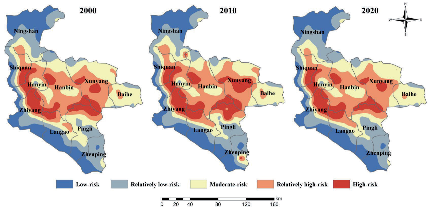
Using the ArcGIS zoning statistics tool, the average values of the LERI in Ankang in 2000, 2010, and 2020 were 0.1627, 0.1670, and 0.1609, respectively, exhibiting an overall trend of an increase before a decline. Thus, the environment in the region demonstrated an increasing trend of resistance to external disturbances. As shown in Fig. 4, the risk level of landscape ecological pattern in the study area during the three periods remained relatively consistent in terms of spatial distribution pattern, exhibiting the spatial distribution characteristics of being higher in the northwest and lower in the southeast and higher in the middle and lower in the surrounding areas, albeit with some differences in the area and number of ecological risk levels. For 20 years, low-risk and relatively low-risk zones in the study area were mainly distributed in strips in the northwestern, western, and southern parts of Ankang. Moderate-risk zones were primarily distributed in strips in the north, central, and south of Ankang. Relatively high-risk zones were largely located in the central region. High-risk zones were mostly distributed in strips in the western part of Ankang and in clusters in the eastern part of the study area.
As shown in Table 4, certain differences were noted in LER levels and their corresponding area percentages across the three periods in the study area. In 2000, 2010, and 2020, the areas of low-risk zones further increased, reaching values of 4200.40, 4225.50, and 4283.16 km2, respectively. The areas of relatively low-risk zones decreased before increasing, reaching values of 4200.40, 4225.50, and 4283.16 km2, respectively. Moderate-risk zones were the largest in terms of area and proportion during the three periods and also exhibited a trend of decreasing before increasing, reaching values of 6043.63, 5454.21, and 5729.74 km2, respectively. The areas of both relatively high-risk and high-risk zones tended to increase before decreasing, reaching values of 5047.95, 5248.10, and 5077.05 km2, and 2788.82, 3493.55, and 2628.22 km2, respectively.
Spatial Statistical Analysis of Landscape Ecological Risks
Global Spatial Autocorrelation Analysis
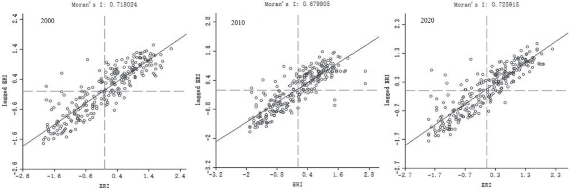
GeoDa 9.5 was used to derive the scatter plot of global Moran’s I values to visualize the spatial distribution of the LERI in 2000, 2010, and 2020 in the 263 risk units in Ankang (Fig. 4). In addition, the spatial distribution pattern and degree of spatial dependence of ecological risks in the region were further verified. The global Moran’s I values of LER in the study area during 2000, 2010, and 2020 were 0.7180, 06799, and 0.7259, respectively. The landscape ecological risk index values were all positive, indicating a positive correlation between landscape ecological risks in the study area. The global Moran’s I values showed a fluctuating increasing trend, indicating that the LERs in Ankang exhibited positive spatial autocorrelation characteristics, implying a spatial aggregation effect. Moreover, the degree of spatial aggregation increased gradually. Overall, areas with high LER values (high–high) have relatively high LER values around them, whereas areas with low LER values (low–low) have relatively low LER values around them.
Local Spatial Autocorrelation Analysis
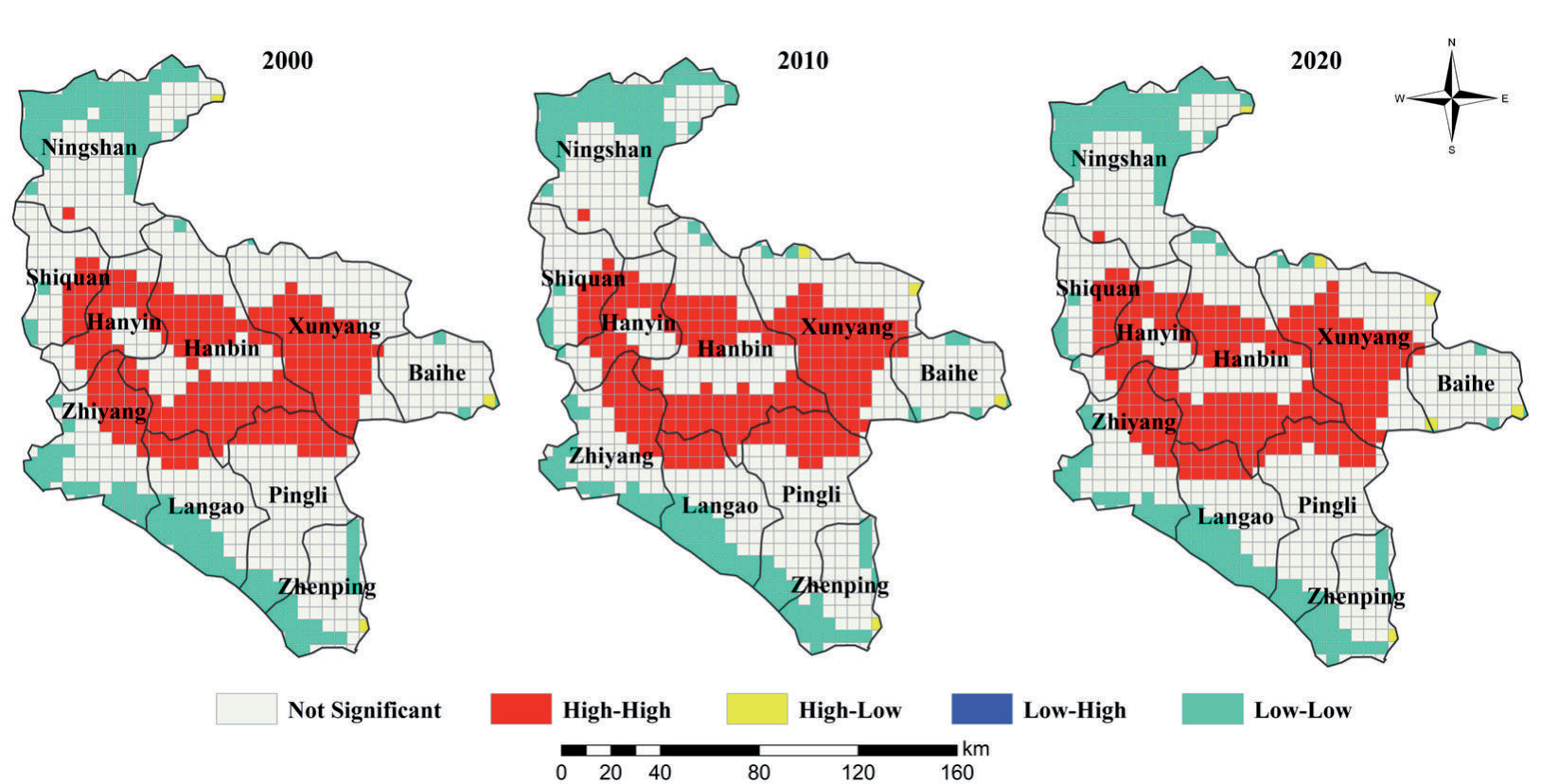
The local indicators of spatial autocorrelation (LISA) were used to further analyze the local spatial aggregation characteristics of LERs in the study area and create a LISA map (Fig. 5). Spatially, for most areas, LER in the study area closely corresponded to the local physical or human geography (population size, GDP, urbanization level, and land development intensity, among others). The level of spatial aggregation of human activities corresponded to that of ecological risk. The spatial aggregation pattern of LER in the study area was primarily of the high–high (H–H) or low– low (L–L) type. Areas with the H–H type of LER were primarily distributed in river valleys (such as in Shiquan County, Hanyin County, and Hanbin District) with flat topography and low vegetation cover and in regions with dense population, fast economic development, high urbanization level, and frequent human activities. Areas with the L–L type of LER were primarily distributed in regions with high topography, high vegetation cover, and little human interference, including sparsely populated parts, relatively backward economic development, and low urbanization levels (such as in the Ningshaan, Xunyang, and Baihe counties, among others). Regions with the L–H type of LERs were scattered in areas such as Ningshaan County, Hanyin County, Hanbin District, and Pingli County. In addition, regions with the H–H and L–L types of LERs showed a gradual clustering trend with time, which is consistent with the kriging interpolation results of the LERI during the same period.
Table 4.
The area statistics of LER grade in the study area.
Standard Deviation Ellipse Analysis
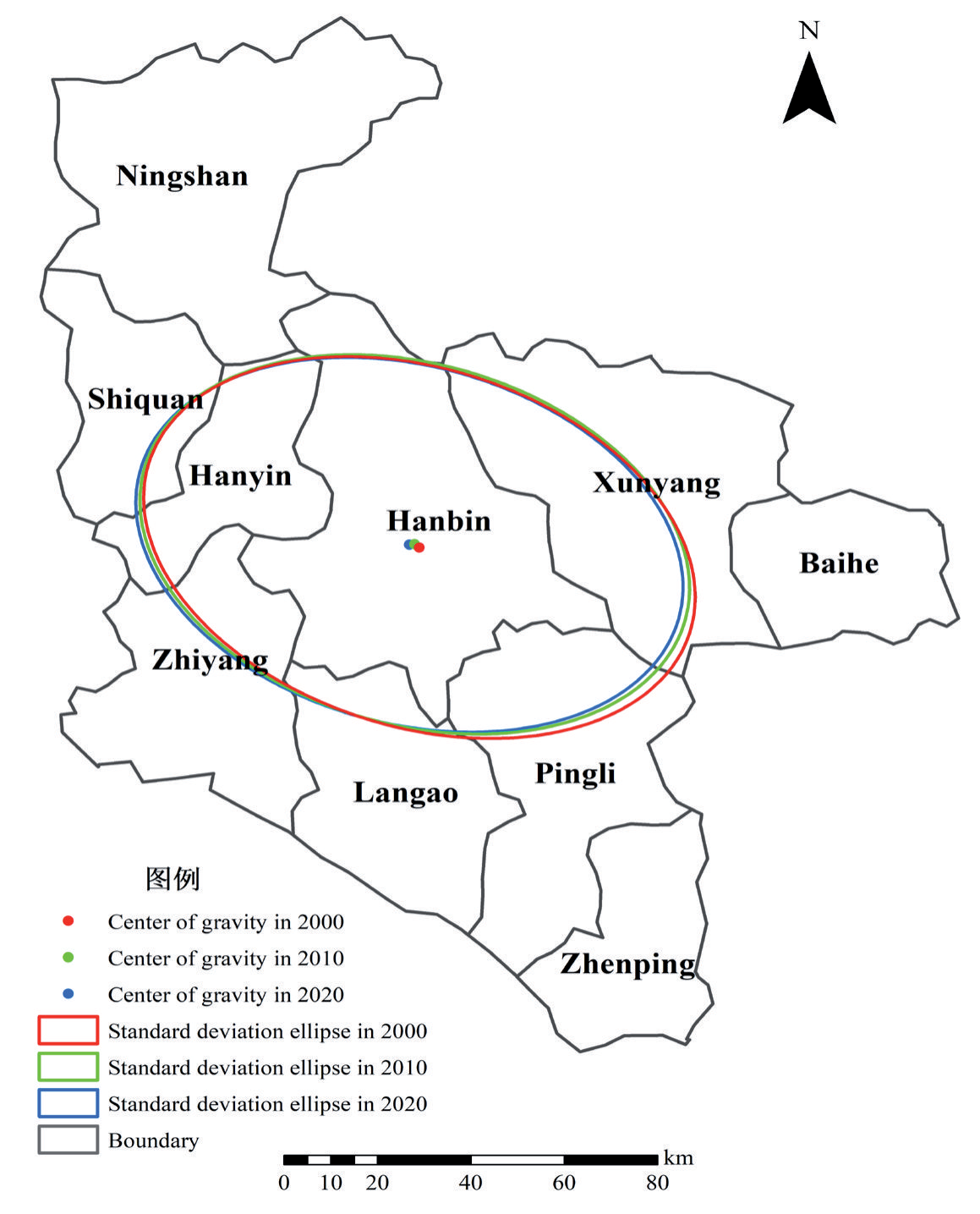
Using directional distribution in the ArcGIS spatial statistics tool, the gravity center and standard deviation ellipse (SDE) of LERIs were calculated during the three periods in the study area. The results are shown in Fig. 6 and Table 5. Comparative analysis of the trajectory of the gravity center of LERs in the study area during 2000, 2010, and 2020 suggested that the gravity center was located in Hanbin District, exhibiting a distribution trend of a shift from the southeast to the northwest. Overall, the gravity center of LER shifted by 1240.95 m from the southeast to the northwest first during 2000-2010 and then by 1141.29 m from the northeast to the southwest during 2010-2020. Therefore, the range of landscape risk changes in the study area was more evident during the early period than during the latter period. From 2000 to 2010, both the major and minor axes showed a decreasing trend, and the ellipticity values of the three periods were 0.6755, 0.6885, and 0.6869, respectively. The ratio between the semi-minor and semi-major axes increased gradually, indicating that the LERI in the study area showed concentrated contraction in the southeast–northwest direction. Moreover, the contraction trend of the major axis was stronger than that of the minor axis, implying that the spatial clustering and convergence of ecological risks gradually increased.
Table 5.
The gravity and standard deviational ellipse of ecological risks in the study area from 2000-2020.
Drivers of Landscape Ecological Risk
Based on all the independent variables, the cross-validation metrics, including MAE, RMSE, and R2, were used to evaluate the model performance of the BRT model in simulating the LERI (Table 6). As shown in Table 6, the average values of MAE in 2000, 2010, and 2020 were 0.040, 0.050, and 0.043, respectively. The average values of RMSE in 2000, 2010, and 2020 were 0.053, 0.068, and 0.057, respectively. The average values of R2 in 2000, 2010, and 2020 were 0.517, 0.438, and 0.568, indicating that the model can explain 51.7%, 43.9%, and 56.8% of the total variability in the LERI, respectively. Overall, the results suggest that the BRT models produced acceptable results in predicting the LERI for the three periods, especially for 2020.
Table 6.
Tenfold cross-validation results of LERI for the BRT model.
| Year | MAE | RMSE | R2 |
|---|---|---|---|
| 2000 | 0.040 | 0.053 | 0.517 |
| 2010 | 0.050 | 0.069 | 0.439 |
| 2020 | 0.043 | 0.053 | 0.568 |
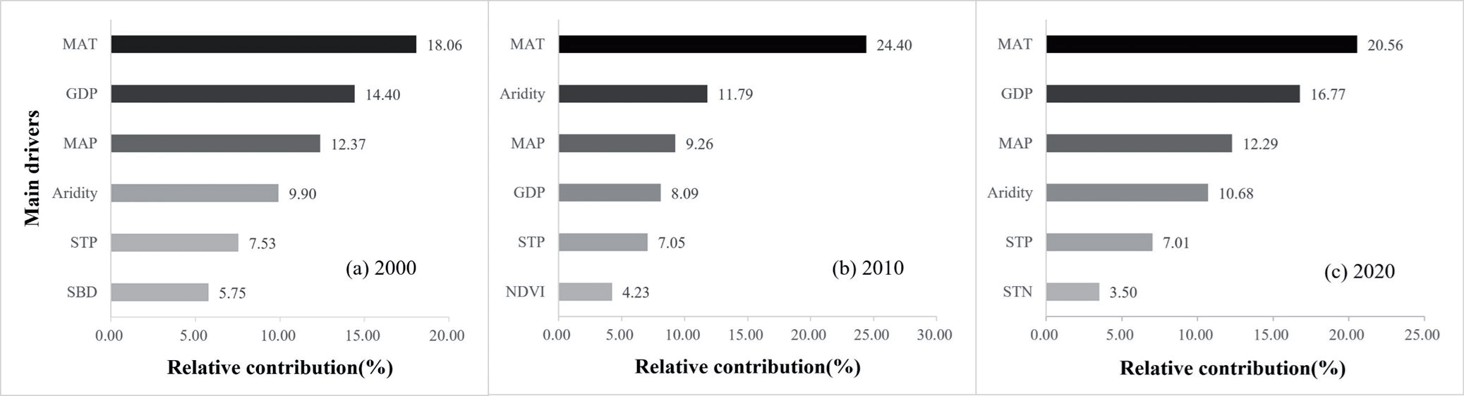
In the present study, 23 drivers covering topography, vegetation cover, climate, socioeconomic, and soil properties that affect the spatial pattern of LERs in the study area were identified and screened using the BRT algorithm. The relative degree of impact of the primary drivers of LERs in the region was obtained from 2000 to 2020. As shown in Fig. 7, the primary drivers affecting the LER pattern in 2000 were MAT, GDP, MAP, aridity, STP, and SBD, with relative contributions of 18.06%, 14.40%, 12.37%, 9.90%, 7.53%, and 5.75%, respectively. The main drivers of LER in 2010 were MAT, aridity, MAP, GDP, STP, and NDVI, with relative contributions of 24.40%, 11.79%, 9.26%, 8.09%, 7.05%, and 4.23%, respectively. The major drivers of LER in 2020 were MAT, GDP, MAP, aridity, STP, and STN, with relative contributions of 20.56%, 16.77%, 12.29%, 10.68%, 7.01%, and 3.50%, respectively. Therefore, MAT, GDP, MAP, aridity, and STP are the primary drivers of LERs in the study area from 2000 to 2020, while natural conditions (mainly climate factors) are the dominant factors shaping the spatiotemporal evolution of LER. The effects of human economic activities on LER in the study area show a trend of decreasing and then increasing over time.
Discussion
Spatiotemporal Evolution Characteristic of the LERI
The spatial heterogeneity of LER is a widely discussed topic by researchers, as it reflects the heterogeneity and complexity of landscape patterns and ecological variables in spatial distribution to a large extent [106, 107]. LER has usually been used to assess the spatiotemporal distribution and evolution characteristics of regional landscape features based on land use and cover change, which also provides an effective and convenient approach for regional ecological risk and environmental quality assessment based on geographic patterns [42, 108-110]. In this study, although the LER method has shown its effectiveness and superiority in quantifying spatiotemporal variability in LER assessment, there are some significant uncertainties in this method due to the differences in the precision of various land use products and the types of evaluation indicators and their weights. Therefore, the uncertainties caused by these factors can also affect the results of regional LER assessments. Despite the above uncertainties, this present study used the most widely accepted method for ecological risk assessment to elucidate the impact of LULC changes on LER, which can provide valuable references for the delineation of ecological protection red lines and nature reserve planning [6, 19, 39, 46, 69, 82, 99, 107, 111].
The spatial distribution pattern of LER in the study area during the three periods showed a high northwest and a low southeast pattern, with a high in the middle and a low in the surrounding areas. From 2000 to 2020, the gravity centers of LER were located in the Hanbin District, with trends of southeast to northwest shift and concentrated contraction. This can be primarily explained as follows: First, the study area is located along the northern slope of the Bashan Mountains in the south and the main ridge of the Qinling Mountains in the north, exhibiting the terrain features of high altitude in the northwest and low altitude in the southeast, as well as low altitude in the surroundings and high altitude in the middle. In addition, various types of vegetation are present in the northwestern and southeastern areas, with widespread woodland areas and high vegetation coverage. However, the vegetation coverage in the northwestern part (i.e., the southern slope of the Qinling Mountains) is significantly higher than that in the southeastern part, and the overall ecological risk shifts toward the northwest of the study area. Second, the geomorphological features of Ankang include high mountains in the north and south and valley basins in the middle. Owing to these features, population and industry are concentrated in the valley basin on both sides of the Hanjiang River – the core area of the Hanjiang Ecological Economic Belt – which is also the focus of economic development in Ankang. Moreover, the landscape type is dominated by arable and construction land, with more frequent disturbances from human activities and greater changes in land use structure, particularly construction land occupying cropland, woodlands, and grassland, among others, which have raised the ecological risk level and induced a shift in risk from the southeast to the northwest. Finally, the scope of the Ankang Qinling Ecological Protection Red Line and Ecological Function Area Plan primarily involves Ningxia County, Shiquan County, Xunyang County, and Hanbin District, as well as other Qinling areas, which also exhibited a northwest–southeast spatial distribution pattern, inducing a gradual shift in the ecological risk of the study area in the northwest direction.
Fig. 8.
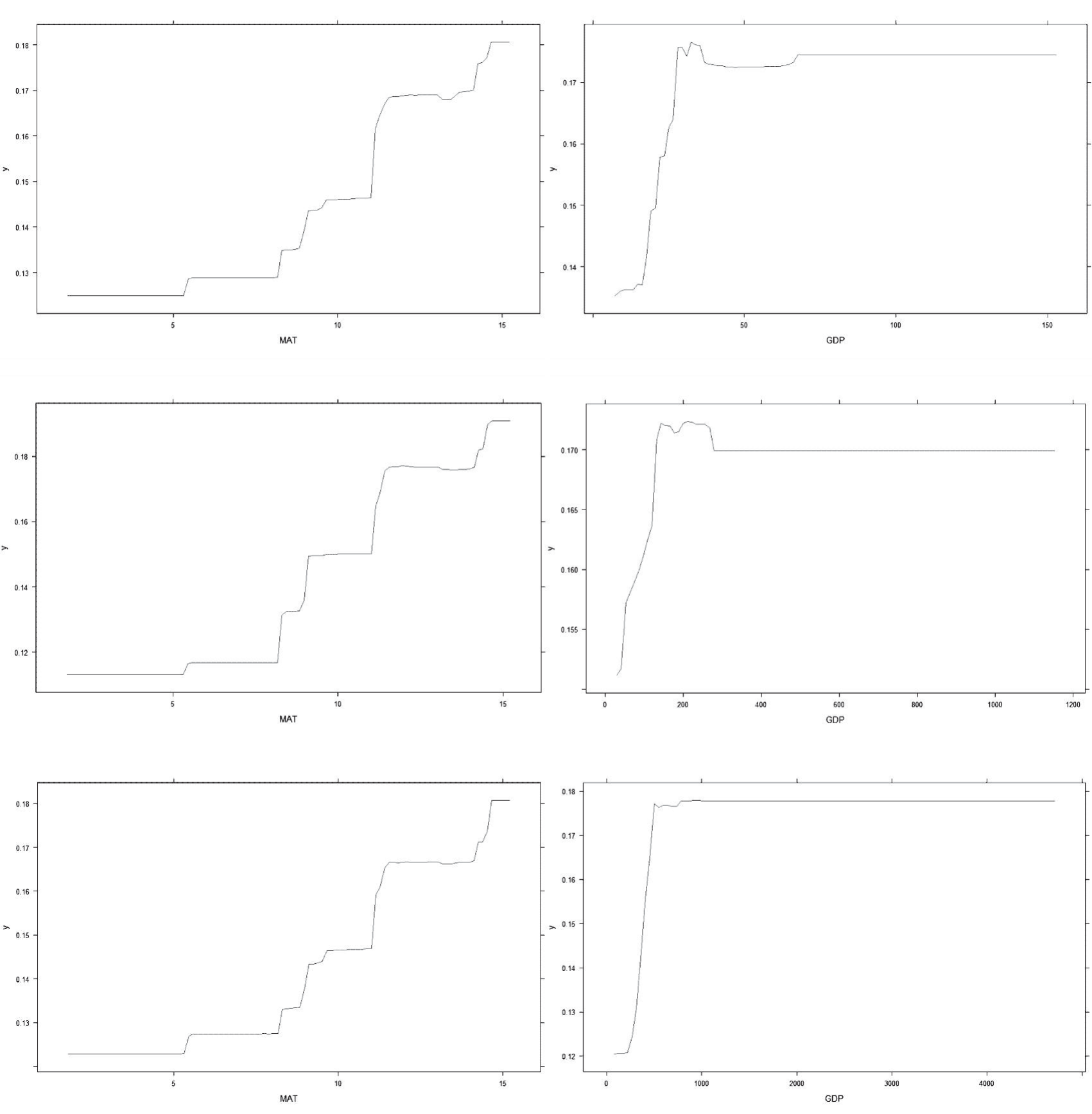
The dynamic response relationships of MAT and GDP to LER in 2000, 2010, and 2020, respectively.
Landscape pattern ecological risk characterizes the impact of human activities on the ecological environment [24, 100, 101, 112]. With the rapid development of urbanization and industrialization, the land use structure and composition of Ankang City have changed dramatically from 2000 to 2020, which inevitably has a great impact on the regional landscape patterns and its ecological risk. Our study concludes that the changes in LERI levels in the study area have gone through two phases. The LERI of the study area increased from 2000 to 2010, while the LERI decreased from 2010 to 2020. This result is consistent with that of [24], who found that the LERI in China’s coastal areas also experienced an increasing and then decreasing trend from 1990-2015. The reason may be that natural/semi-natural landscapes such as croplands, forests, and waters are prone to being occupied and destroyed by human production and living activities during the advancement of urbanization, which has led to an increase in landscape fragmentation, separation, and loss of these land-use types in the past 20 years. Our results are also supported by previous literature [26, 36, 40, 92]. As a key ecological function area and vital ecological protection barrier in China, the region showed an overall downward but fluctuating trend of LER from 2000 to 2020. This result directly reflects that China’s long-term strategic goal of promoting “ecological civilization” has achieved remarkable outcomes and created conditions conducive to improving the ecological environment and landscape ecosystem in the Qinling–Bashan Mountains.
Key Drivers of Spatiotemporal Variation in the LER
Unlike previous literature on the selection of drivers of spatiotemporal changes in LER [42, 99, 111, 113- 115], this study not only adopted regular drivers such as topography, climate, vegetation, and human activities, but also innovatively incorporated soil physicochemical properties into the BRT model to further explore the driving mechanism of LER. Among the 23 drivers, our results indicated that MAT and GDP were the most important drivers in Ankang City during the study period, followed by MAP, aridity, and STP, which were the primary drivers of LER. Although distinct drivers in the study area produced different degrees of impact on LER during the three periods, attribution analysis revealed that climatic factors (e.g., MAT, MAP, and aridity), socio-economic activities (e.g., GDP), and soil properties (e.g., STN, STP, and SBD) play an important role in the spatiotemporal variation of LER in the study area, indicating that the spatial pattern of LER in this region is shaped by a combination of natural conditions and human activities. These results were consistent with the semi-variance function results. These findings of the present study are consistent with those of the previous report in the Weibei rainfed highlands of Shaanxi Province [116]. Gao et al. [57] observed that spatiotemporal patterns of LER in the Sichuan–Yunnan ecological barrier area from 2000-2020 were affected by natural factors, such as elevation, precipitation, population, and GDP, as well as anthropogenic activities, although natural factors were the dominant drivers, consistent with the findings of the present study. In addition, we also used the BRT model to reveal the nonlinear response relationship of different drivers to LER over the past 20 years (Fig. 8), which provided more detailed information to explore the driving mechanism of the dynamic changes of LER. However, due to the limited space, here we only show the dynamic relationship between MAT and GDP in response to LER in 2000, 2010, and 2020, respectively (Fig. 8). Based on the effects of different drivers on LER, we found that LER fluctuates with explanatory variables, especially for the key drivers. Moreover, LER increased with the increase of MAT, MAP, aridity, GDP, PD, and pH from 2000 to 2020, which also indicated that they exacerbated the ecological degradation in the study area. On the contrary, LER decreased with the increase of NDVI, ST, CF, STH, STN, STP, and STK. Moreover, we found that the LER fluctuated with the explanatory variables, especially the key drivers. This finding also suggested that LER in the study area was sensitive to changes in key drivers, which requires the government to pay special attention to the effects of changes in climate, soil properties, and socio-economic development when implementing ecological environmental protection and management in the future.
Although the national policy factor is difficult to quantify, it profoundly affects the spatial pattern of LER [42, 117-122]. From 2000 to 2020, the degree of industrialization in the study area increased significantly, and rapid economic development accelerated the urbanization process, leading to an increase in the scale and demand for construction land. Moreover, the implementation of policies aimed at returning farmland to forest, farmland to grassland, grazing land to grassland, and comprehensive land improvement has triggered significant changes in the rational allocation of land resources, which has led to the optimization and modification of the land use structure to a large extent. From 2000 to 2010, against the background of the reform of the socialist market economy system and the development strategy of Western China, the population, economy, and urbanization rate of the study area have increased sharply, and infrastructure construction has been strengthened, resulting in the occupation of cropland, woodland, and grassland for construction. Moreover, ecological damage, such as vegetation destruction, arable land destruction, soil erosion, surface source pollution, and biodiversity loss, has worsened ecological risks. However, since 2010, the Shaanxi provincial and Ankang municipal governments have issued a series of plans related to the ecological protection of the Qinling Mountains in Ankang, implementing the strictest ecological protection systems and adopting measures such as grazing prohibition, forestation, forest, and grassland restoration, water resources protection, water body management, natural resource development control, ecological restoration, and treatment, among others. The implementation of these measures strengthened the ability of ecosystems to withstand external disturbances, thereby minimizing the overall ecological risk. Therefore, over time, the LERI of the study area showed an overall upward trend, followed by a decline.
Policy Implications
Over the past 20 years, the degree of impact of anthropogenic activities (notably economic development) on the ecological risk of landscapes has become stronger, accelerating changes in the spatial structure of the country and landscape types. Moreover, the evolution of the structure and quality of landscape types, primarily woodlands, grasslands, and croplands, is the key to the stability of ecological functions in the study area. Therefore, to prevent further deterioration of the ecological environment in this region, more attention must be paid to the impacts of climate change and human activities on the ecosystem, especially issues such as ecosystem degradation and eco-environment destruction caused by the process of economic development in the context of extreme climate. Meanwhile, the government can improve water and temperature conditions as well as soil fertility in the study area through afforestation, forestation and grassland rehabilitation, ecological restoration, comprehensive land and space improvement, land and space assessment, optimal land allocation, and land and space structure optimization to reduce the degree of LERs and improve the quality of the ecological environment in the study area. Furthermore, the local government should transform the economic development model and establish a robust economic system featuring sustainable, low-carbon, and circular development to promote and achieve high-quality development of the regional economy as well as sustainable development.
Limitations and Future Prospects
Based on multi-source geographical data, this study systematically investigated the spatiotemporal variations and main drivers of LER in the Ankang City of Qinling-Daba Mountains region in China using the BRT model, which provides not only scientific guidelines for ecological assessment and policy formulation in other ecologically fragile regions in China, but also a practical reference for the coupling and coordination between socio-economic development and ecological environmental protection in ecologically sensitive regions. Although this study has improved our understanding of the driving mechanisms governing the spatiotemporal distribution of LER in the study area, it still has several limitations and challenges that we plan to overcome in further research.
First, similar to most relevant studies [15, 23, 26, 40, 53, 55, 64, 69, 107, 110, 117-122], the landscape disturbance index, landscape vulnerability index, and landscape loss index mainly depend on the experts’ prior knowledge and subjective experience in this study, which may affect the weight allocation of LER and thus the spatiotemporal pattern of LER. Therefore, objective methods such as the analytic hierarchy process, entropy weighting, principal component analysis, the technique for order preference by similarity to the ideal solution, and the gray correlation method can be used to assign the weights of LER in our future research.
Second, owing to the obvious spatial heterogeneity and extensive scale/granularity dependence in landscape patterns, the grid size of LER units largely influences the spatial pattern of LER [101]. However, this study had a relatively single spatial scale and did not investigate the spatiotemporal variability and the drivers of LER at different spatial scales. Hence, we plan to set multiple spatial scales to select the best risk units so that the spatial pattern of LER can be constructed and optimized.
Third, due to the availability of data, the accuracy of the topographic factor and other drivers with a spatial granularity of 90 m and 1000 m, respectively, may be low, which is likely to weaken or mask the influence of explanatory variables on the spatial pattern of LER and thus draw different conclusions. As a result, it is necessary to use high spatial resolution and in situ observation data to quantitatively reveal the response relationship of different drivers to LER.
Finally, because of the complexity and diversity of ecosystems and ecological environments in the Qinling-Daba Mountain region, how land use, ecological risk, and ecological environments in the study area will change remains elusive in the future. Thus, in the future, ecological service evaluation and land use modeling can be incorporated into the assessment and prediction of LER to better serve the local government in the decision-making and management of ecological environment restoration and protection.
Conclusions
In this study, we thoroughly investigated the spatiotemporal dynamics of land use and LERI in a typical region of the Qinling-Dabashan Mountains, and then the driving mechanisms of spatial distribution for LERI were systematically analyzed based on the BRT model. The results indicated that: (1) Woodland and cropland were the primary land use types that were converted from 2000 to 2020. Woodland was primarily converted to cropland, grassland, and construction land, while cropland was primarily converted to woodland, grassland, and construction land. The land use changes were affected by urbanization levels and economic development. (2) Overall, during the past 20 years, the LERI has followed an upward trend, followed by a decline, indicating that the ecological environment of the region has been gradually improved and has the ability to resist external disturbances. (3) The spatial pattern of LER level has remained relatively consistent during the three periods, with the distribution characteristics being high in the northwest, low in the southeast, high in the middle, and low in the surrounding areas. (4) The global Moran’s I values of LERI from 2000 to 2020 exhibited a fluctuating upward trend with significant spatial positive correlation clustering characteristics. The LISA maps of LERI were similar to those of the spatial distribution pattern, and the clustering patterns were primarily of the H–H and L–L types. (5) Standard deviation ellipse analysis indicated that all gravity centers of LERs from 2000 to 2020 were in Hanbin District, Ankang. However, the concentrated contraction was noted in the southeast– northwest direction, and the contraction trend of the major axis was stronger than that of the minor axis. (6) MAT, GDP, MAP, aridity, and STP were the primary drivers of spatial distribution for LERs during the study period, and the impact of human economic activities on LERs shows a trend of decreasing and then increasing over time. Our results strengthen our understanding of the influence of anthropogenic and natural factors, especially climate and economic activities, on landscape management and even the ecological environment and provide practical guidance for future ecological risk prevention and sustainable development of landscapes under different climatic and anthropogenic changes.

